Cardinality Estimation Feedback in SQL Server 2022

Part of the SQL Server 2022 blog series.

Cardinality estimation (CE) is a process used by the query optimizer to estimate the number of rows returned by a query or sub-part of a query. These estimates rely on two underlying things: statistics about the data and a set of assumptions—known as the model. The model determines how we interpret statistics and data coming from various sub expressions, and so, for any given set of statistics, different models will arrive at different cardinality estimates. 

Until SQL Server 2022, CE could only have one model. The set of assumptions used was baked into the code of the server, and so whatever model was picked is what was used for all queries. However, we know that not all queries and workloads perform best under one single model. For some queries, the model we use works out well, but for others, a different model would perform better. With CE Feedback in SQL Server 2022, we can now tailor the model used to generate a query play to the specific query.

CE has always had three basic assumptions that comprise the model: independence (or partial independence), uniformity, and containment. These three assumptions determine how we interpret histograms, and they determine how we combine data during joins or in the presence of multiple predicates. In this blog, I will explain these model variants and what they mean in more detail.

Uniformity

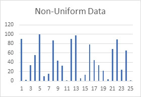
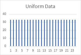
Let’s begin by discussing uniformity assumption. This assumption is used when interpreting data from the on-disk histograms—abstracted data about the columns being queried. We assume that all data within steps, or buckets, of a histogram is uniformly distributed at an average frequency for that bucket. Thus, when we query data, this allows us to determine the number of rows that satisfy the predicate. 

Now, CE Feedback modifies the uniformity assumption only in one special case—that of Row Goal queries. These queries look like TOP n, or Fast n, or IN. and there is a special optimization for row goal queries that relies on the independence assumption. Whenever we believe that a particular value occurs at a high enough frequency (based on our interpretation of the histogram using the independence assumption), we choose to do a quick scan of a few pages assuming that we will get enough qualifying rows very quickly. However, if the data is skewed, we may have falsely assumed more qualifying values than were actually present. This means we scan far more pages than expected to get the requisite number of rows.

Independence

Consider a where clause with two predicates, combined with an AND. Something like City=’Seattle” AND State=’WA’. Under the model assumption of independence, we would take the selectivity of the individual predicates (City=’Seattle’, State=’WA’) and multiply those probabilities together. Under the model assumption of correlation, we would take the most selective predicate (City=’Seattle’) and use the selectivity of that predicate only to determine the selectivity of the conjunctive clause. There is a third model of partial correlation, in which we multiply the selectivity of the most selective predicate with a weakened selectivity (raised to a power less than 1, to make the selectivity closer to 1) of the successive predicates. 

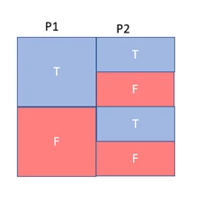
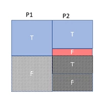
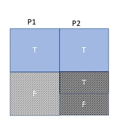
CE always starts out with this last model of partial independence (referenced in other places as exponential backoff), but with CE Feedback, we can see if our estimates are too high, meaning the predicates are more independent, or too low, meaning that there is more correlation than expected, and adjust the model used for that query and those predicates accordingly for future executions. If this makes the plan or performance better, we persist this adjustment using a query store hint, and use it for future executions.

Containment

The model assumption of containment means that users query data that is actually in the table. Meaning, if there is a column = constant predicate in the table, we assume that the constant actually exists in the table, at the frequency appropriate for where it falls within the histogram. However, we also assume that there is a containment relationship between joins. Basically, we assume that users wouldn’t join two tables together if they didn’t think there would be matches. However, there are two ways of looking at the containment relationship between joins: Base containment, or Simple containment.

Base containment assumes that there is an inherent relationship between the tables participating in a join but doesn’t make assumptions about the filters occurring on top of those tables before the join occurs. A good example might be a table of store sales and a table of store returns. We would assume that all things returned were also sold, but we would not assume that any filtering on the sales or returns tables makes containment more or less likely—we just assume containment at the base table level and scale the size of the estimated result up or down based on the filters in play.

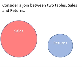
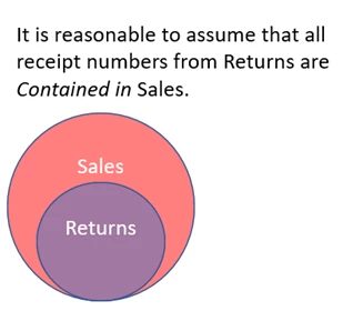
Simple containment is a bit different—instead of assuming some inherent relationship between the base tables, it assumes that the filters applied to those tables create a containment relationship. For example, querying for graduating seniors from a specific high school and joining that with a query for athletes in a given zip code. While there is some inherent relationship between the two tables a priori, the filters applied specifically limit and create a containment relationship. 

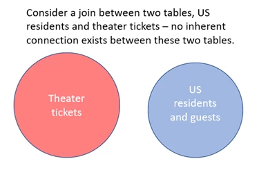
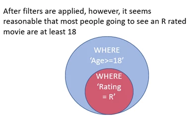
CE starts with the base containment model for all queries. However, if the estimates for the join are ‘off’ in some way—the incoming estimates are good, the outgoing estimates are bad—we try the alternate containment model. When the query is executed again, we try out the other model, and if it is better, we persist it with a query store hint and use it for future executions.

Conclusion

In summary, CE requires a basic set of assumptions that are used to interpret and combine statistical data about histograms or sub-parts of a query. Those assumptions work well for some queries, and less well for others. In SQL Server 2022, we have introduced a method of CE Feedback which adjusts those assumptions in a per-query way, based on actual performance of the query over time. 

Learn more

• See what’s new in SQL Server 2022.
• Try out the Microsoft Learn SQL Server 2022 module and the SQL Server 2022 workshop.