Swin Transformer supports 3-billion-parameter vision models that can train with higher-resolution images for greater task applicability

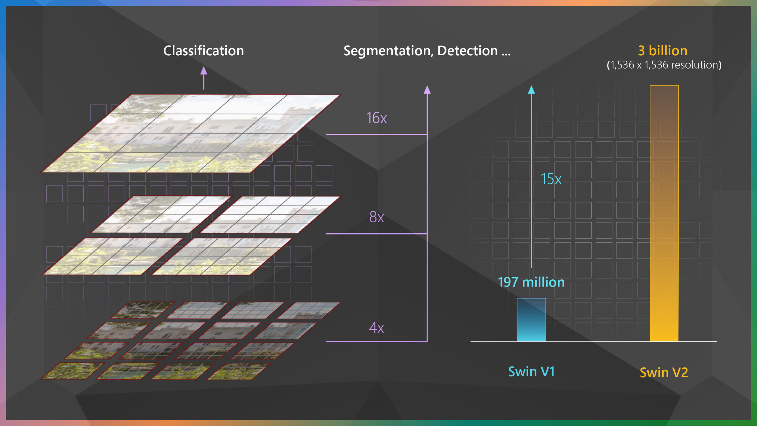
Early last year, our research team from the Visual Computing Group (opens in new tab) introduced Swin Transformer (opens in new tab), a Transformer-based general-purpose computer vision architecture that for the first time beat convolutional neural networks on the important vision benchmark of COCO object detection (opens in new tab) and did so by a large margin. Convolutional neural networks (CNNs) have long been the architecture of choice for classifying images and detecting objects within them, among other key computer vision tasks. Swin Transformer offers an alternative. Leveraging the Transformer architecture’s adaptive computing capability, Swin can achieve higher accuracy. More importantly, Swin Transformer provides an opportunity to unify the architectures in computer vision and natural language processing (NLP), where the Transformer has been the dominant architecture for years and has benefited the field because of its ability to be scaled up.

So far, Swin Transformer has shown early signs of its potential as a strong backbone architecture for a variety of computer vision problems, powering the top entries of many important vision benchmarks such as COCO object detection, ADE20K semantic segmentation, and CelebA-HQ image generation. It has also been well-received by the computer vision research community, garnering the Marr Prize for best paper at the 2021 International Conference on Computer Vision (ICCV). Together with works such as CSWin, Focal Transformer, and CvT, also from teams within Microsoft, Swin is helping to demonstrate the Transformer architecture as a viable option for many vision challenges. However, we believe there’s much work ahead, and we’re on an adventurous journey to explore the full potential of Swin Transformer.

In the past few years, one of the most important discoveries in the field of NLP has been that scaling up model capacity can continually push the state of the art for various NLP tasks, and the larger the model, the better its ability to adapt to new tasks with very little or no training data. Can the same be achieved in computer vision, and if so, how?

In pursuit of answers, we scaled up Swin Transformer to 3 billion parameters, the largest and most effective dense vision model to date. There have been successfully trained vision models with up to 1.8 billion parameters. However, these vision models require billions of labeled images to be trained well and are applicable to only image classification. With our model, SwinV2-G, we address a common obstacle when increasing model size in the computer vision space—training instability—to support more parameters, and thanks to a technique we developed to address the resolution gap that exists between pretraining and fine-tuning tasks, SwinV2-G marks the first time that a billion-scale vision model has been applied to a broader set of vision tasks. Additionally, leveraging a self-supervised pretraining approach we call SimMIM, SwinV2-G uses 40 times less labeled data and 40 times less training time than previous works to drive the learning of billion-scale vision models.

SwinV2-G achieved state-of-the-art accuracy on four representative benchmarks when it was released in November: ImageNetV2 image classification, COCO object detection, ADE20K semantic segmentation, and Kinetics-400 video action classification.

Our experience and lessons learned in exploring the training and application of large vision models are described in two papers—“Swin Transformer V2: Scaling Up Capacity and Resolution” (opens in new tab) and “SimMIM: A Simple Framework for Masked Image Modeling” (opens in new tab)—both of which are being presented at the 2022 Computer Vision and Pattern Recognition Conference (CVPR) (opens in new tab). The code for Swin Transformer (opens in new tab) and the code for SimMIM (opens in new tab) are both available on GitHub. (For the purposes of this blog and our paper, the upgraded Swin Transformer architecture resulting from this work is referred to as V2.)

Improving training stability

The first issue we faced when training large models was the problem of training instability. We observed that as models get larger, it becomes very easy for them to crash. After checking the feature values of each layer of the models we trained in scaling up Swin Transformer to 3 billion parameters, we found the cause of the instability: large feature variance discrepancy between different layers.

As shown in Figure 1, the average feature variance in the deep layers of the original Swin Transformer model increases significantly as the model grows larger. With a 200-million-parameter Swin-L model, the discrepancy between layers with the highest and lowest average feature variance has reached an extreme value of 10^4. Crashing occurs during training when the model capacity is further scaled to 658 million parameters (Swin-H).

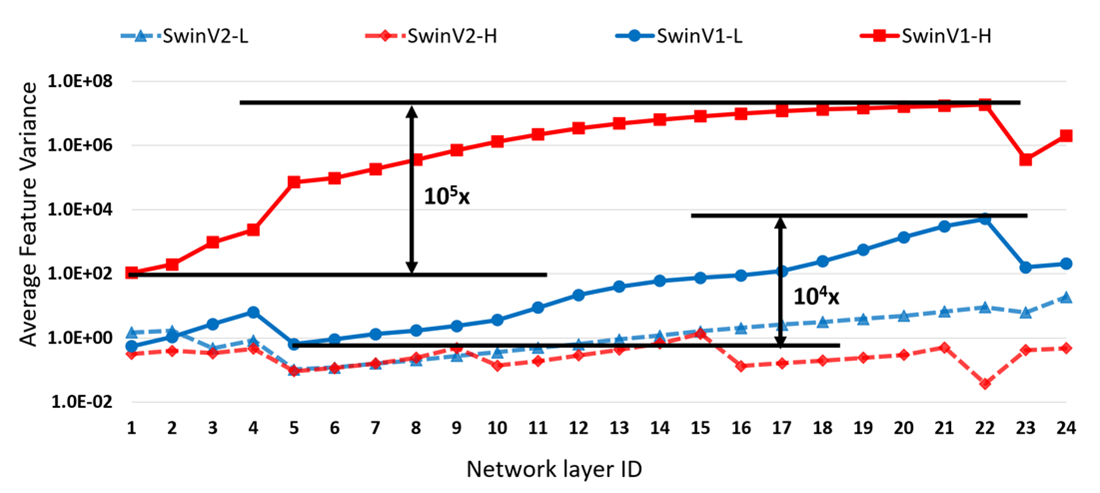
Looking closely at the architecture of the original Swin Transformer, we found that this was due to the output of the residual branch being added directly back to the main branch without normalization. In other words, the unconstrained output feature values could be very large compared to the input. As illustrated in Figure 2 (left), after one Transformer block, the feature values of the output can increase to 61 times larger than that of the input. To alleviate this problem, we propose a new normalization method called residual-post-normalization. As shown in Figure 2 (right), this method moves the normalization layer from the beginning to the end of each residual branch so that the output of each residual branch is normalized before being merged back into the main branch. In this way, the average feature variance of the main branch doesn’t increase significantly as the layers deepen. Experiments have shown that this new normalization method moderates the average feature variance of each layer in the model (see the dashed lines in Figure 1; the SwinV2 models have the same respective number of parameters as the SwinV1 models: 200 million [L] and 658 million [H]).

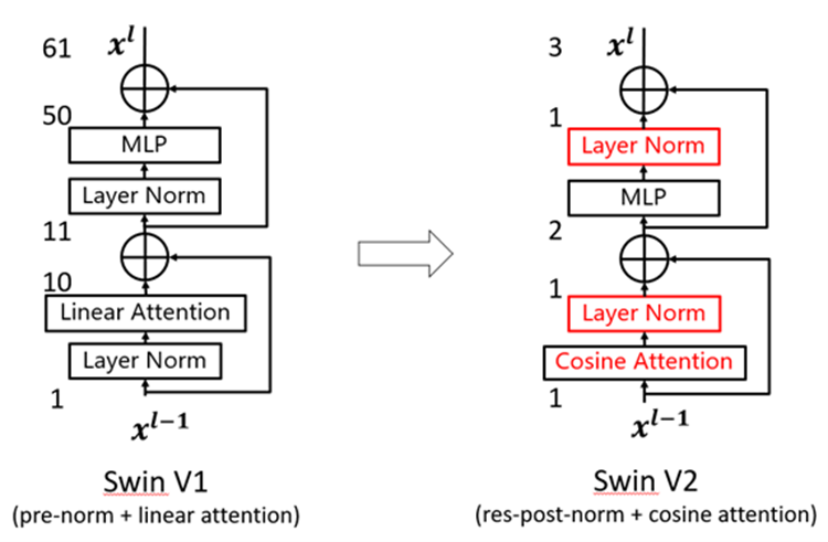
In addition, we also found that as the model becomes larger, the attention weights of certain layers tend to be dominated by a few specific points in the original self-attention computation, especially when residual-post-normalization is used. To tackle this problem, our team further proposes the scaled cosine attention mechanism (see Figure 2 right) to replace the common dot-product linear attention unit (opens in new tab). In the new scaled cosine attention unit, the computation of self-attention is independent of the input magnitude, resulting in less saturated attention weights.

Experiments have shown that residual-post-normalization and the scaled cosine attention mechanism not only stabilize the training dynamics of large models but also improve accuracy.

Addressing large resolution gaps between pretraining and fine-tuning tasks

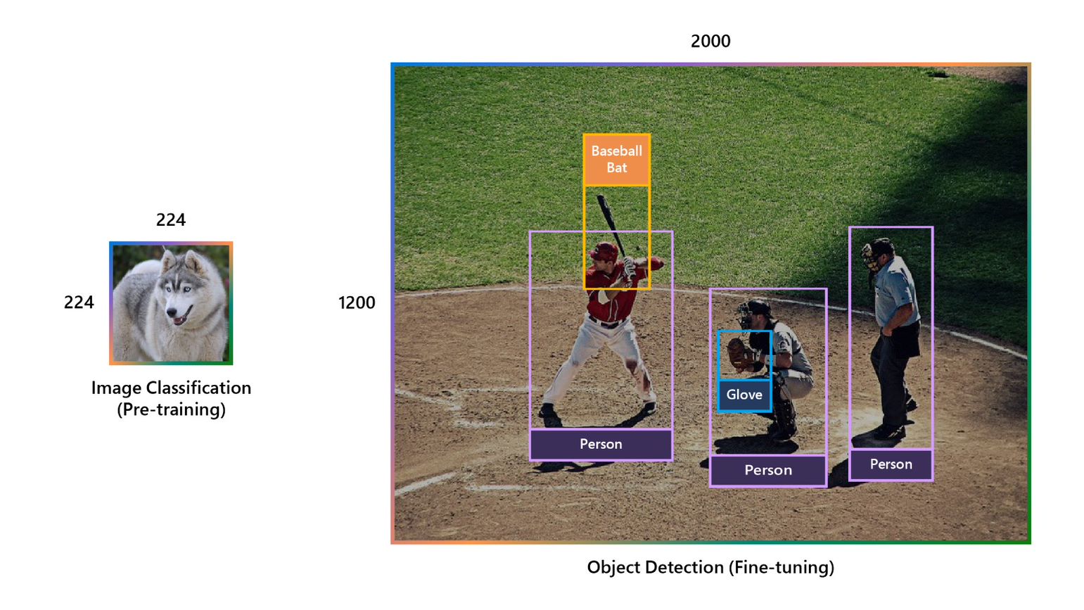
Another difficulty with large vision models is that the image resolution discrepancy between pretraining and fine-tuning can be large: pretraining is typically carried out at low resolutions, while many downstream vision tasks require high-resolution input images or attention windows, as shown in Figure 3.

In Swin Transformer, there’s a term of relative position bias in the attention unit to represent the impact of one image patch on another based on the relative position between them. This term is learned in pretraining. However, since the relative position range at fine-tuning has been changed significantly compared to that in pretraining, we need techniques to initiate the biases at new relative positions not seen in pretraining. While the original Swin Transformer architecture uses a handcrafted bicubic interpolation method to transfer the old relative position biases to the new resolution, we find it’s not that effective when the resolution discrepancy between pretraining and fine-tuning is very large.

To resolve this problem, we propose a log-spaced continuous position bias approach (Log-spaced CPB). By applying a small meta-network to the relative position coordinates in log space, Log-spaced CPB can generate position bias for any coordinate range. Since the meta-network can take arbitrary coordinates as input, a pretrained model can freely transfer between different window sizes by sharing the weights of a meta-network. Moreover, by converting the coordinates to a log space, the extrapolation rate required to transfer between different window resolutions is much smaller than with using the original linear space coordinates.

Using Log-spaced CPB, Swin Transformer V2 achieves smooth transferring between different resolutions, enabling us to use a smaller image resolution—192 × 192—with no accuracy loss on downstream tasks compared with the standard 224 × 224 resolution used in pretraining. This speeds up training by 50 percent.

Scaling model capacity and resolution results in excessive GPU memory consumption for existing vision models. To address the memory issue, we combined several crucial techniques, including Zero-Redundancy Optimizer (ZeRO), activation checkpointing, and a new sequential self-attention implementation. With these techniques, GPU memory consumption is significantly reduced for large-scale models and large resolutions with little impact to training speed. The GPU savings also allows us to train the 3-billion-parameter SwinV2-G model on images with resolutions of up to 1,536 × 1,536 using the 40-gigabyte A100 GPU, making it applicable to a range of vision tasks requiring high resolution, such as object detection.

Tackling the data starvation problem for large vision models

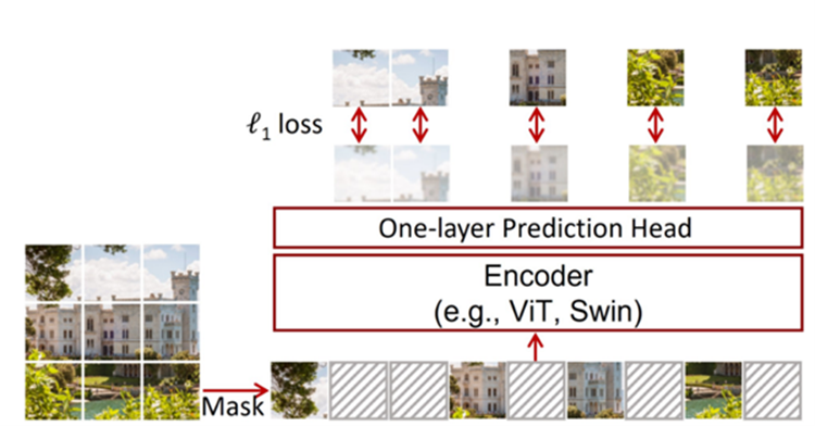
Training larger models often requires more labeled data; however, the computer vision field lacks such labeled data at scale because of the high cost of human-annotated data. This has compelled the vision field to explore the training of large models with smaller amounts of labeled data. To this aim, we introduce the self-supervised pretraining approach SimMIM, short for Simple Framework for Masked Image Modeling.

As shown in Figure 4, SimMIM learns image representation by masked image modeling, a pretext task in which a portion of an input image is masked and then the model predicts the RGB values of the masked area given the other visible parts. By this approach, the rich information contained in each image is better exploited, which allows us to use less data to drive the training of large models. With SimMIM, we were able to train the SwinV2-G model by using only 70 million labeled images, which is 40 times less than that used by previous billion-scale vision models.

Setting new records on four representative vision benchmarks

By scaling up model capacity and resolution, Swin Transformer V2 set new records on four representative vision benchmarks when it was introduced in November: 84.0 percent top-1 accuracy on ImageNetV2 image classification; 63.1 / 54.4 box / mask mean average precision (mAP) on COCO object detection; 59.9 mean Intersection-over-Union (mIoU) on ADE20K semantic segmentation; and 86.8 percent top-1 accuracy on Kinetics-400 video action classification.

Benchmark	ImageNetV2	COCO test-dev	ADE20K val	Kinetics-400
Swin V1	77.5	58.7	53.5	84.9
Previous state of the art	83.3 (Google, July 2021)	61.3 (Microsoft, July 2021)	58.4 (Microsoft, October 2021)	85.4 (Google, October 2021)
Swin V2 (November 2021)	84.0 (+0.7)	63.1 (+1.8)	59.9 (+1.5)	86.8 (+1.4)

We hope this strong performance on a variety of vision tasks can encourage the field to invest more in scaling up vision models and that the provided training “recipe” can facilitate future research in this direction.

To learn more about the Swin Transformer journey, check out our Tech Minutes video (opens in new tab).

Swin Transformer research team

(In alphabetical order) Yue Cao, Li Dong, Baining Guo, Han Hu, Stephen Lin, Yutong Lin, Ze Liu, Jia Ning, Furu Wei, Yixuan Wei, Zhenda Xie, Zhuliang Yao, and Zheng Zhang

（在新选项卡中打开）