Games are popular as a test-bed for new machine learning techniques because they can be very challenging and allow for easy analysis of new learning techniques in a controlled environment. For reinforcement learning, where the goal is to learn good behavior in a data-driven way, the Arcade Learning Environment (ALE), which provides access to a large number of Atari 2600 games, has been a popular test-bed.
In 2015, Mnih et al. achieved a breakthrough in RL research: by combining standard RL techniques with deep neural networks, they outperformed humans on a large number of ALE games. Since then, many new methods have been developed based on the same principles, improving performance even further. Nonetheless, for some of the ALE games, DQN and its successors are unsuccessful, achieving only a fraction of the score that a human gets. One of these hard games is the classical game Ms. Pac-Man.
As reasons for why some games are hard often sparse-reward issues or partial observability are mentioned. However, these `usual suspects’ do not seem to apply to Pac-Man: there are plenty of rewards in the game and the game is fully observable. Hence, an interesting question arises: what is it that makes the game Ms. Pac-Man hard for learning methods?
on-demand event
In our blog post we look deeper into the reason for why Ms. Pac-Man is hard and propose a new technique, called Hybrid Reward Architecture, to deal with the underlying challenge of Ms. Pac-Man.
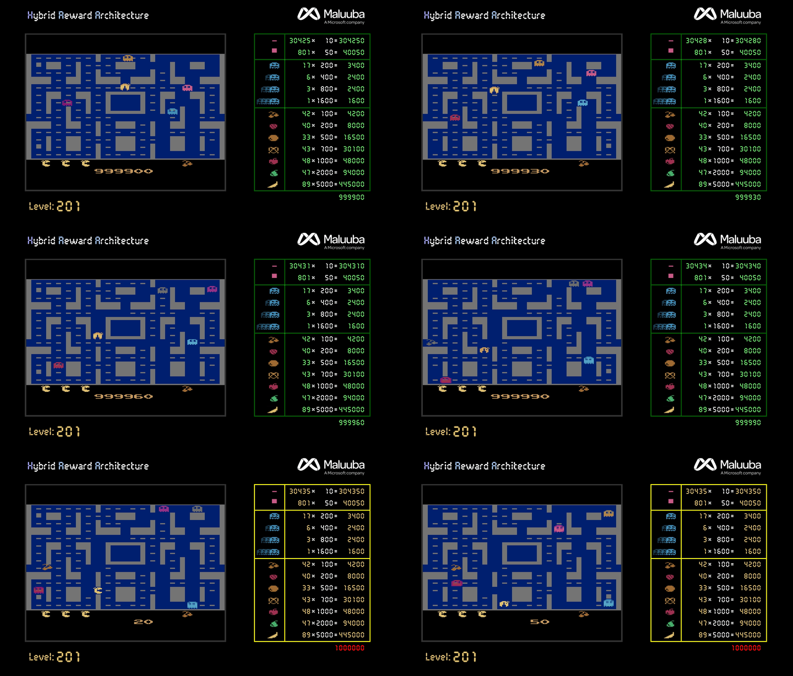
Using this technique we were able to achieve the maximum possible score of 999,990 points.

The challenge
Before we can address the question of why Ms. Pac-Man is a hard game for learning methods, we have to place it in the right context. If we consider unlimited resources, that is, unlimited computation time, memory and interactions with the game, learning a good policy is easy: storing an exact value for each individual frame and using standard RL methods like Q-learning, will over time yield the optimal policy. The challenge lies in learning a policy efficiently. In the DQN paper, efficient learning is (somewhat arbitrarily) defined as at most 800 million game interactions. This might seem like a large number (it corresponds with close to 4000 hours of real-time game-play), compared to the number of possible game states that can be encountered—up to 10^77 for Ms. Pac-Man—it is an extremely tiny amount. This necessarily means that strong generalization is required to learn an effective policy.
Generalization
In the context of behavior policies, generalization refers to being able to come up with effective policies for new situations by leveraging experiences on different, but related situations. Humans are extremely good in this. For example, we are able to reliably pick up a cup and drink from it, in all kinds of different situations. Even in a place we have never been before, and with a cup we have never seen before, we can effortlessly take a sip. While this type of generalization is trivial for humans, for learning algorithms it is one of the biggest challenges.
In (deep) RL, generalization of behavior typically occurs via the value function. A value function gives the expected sum of rewards under a particular policy and plays an important role when trying to find a good policy. Specifically, by incrementally improving estimates of the optimal value function, behavior can be improved. By using a deep neural network for representing the value function, generalization of the value function occurs, and hence of the policy.
However, when the optimal value function is very complex, learning a low-dimensional representation can be challenging or even impossible. For such domains, we propose to use an alternative value function that is smoother and can be more easily approximated by a low-dimensional representation.
Performance metric vs learning objective
A key observation behind our approach is the difference between performance objective, which specifies what type of behavior is desired, and the training objective, which provides the feedback signal that modifies an agent’s behavior. In RL, a single reward function often takes on both roles. However, the reward function that encodes the performance objective might be very bad as a training objective, resulting in slow or unstable learning. At the same time, a training objective can be very different from the performance objective but still do well with respect to it.
Decomposition of reward function
Our main strategy for constructing a training objective is to decompose the reward function of the environment into n different reward functions. Each of them is assigned to a separate reinforcement-learning agent. All these agents can learn in parallel on the same sample sequence by using off-policy learning. For action selection (as shown in Figure 1), each agent gives its values for the actions of the current state to an aggregator, which combines them into a single action-value for each action (for example, by averaging over all agents). Based on these action-values the current action is selected.

Figure 1
Decomposition for Ms. Pac-Man
In the Atari game Ms. Pac-Man points are obtained by eating pellets, while avoiding ghosts (contact with one causes Ms. Pac-Man to lose a life). Eating one of the special power pellets turns the ghosts blue for a small duration, allowing them to be eaten for extra points. Bonus fruits can be eaten for further points, twice per level. When all pellets have been eaten, a new level is started. There are a total of 4 different maps and 7 different fruit types, each with a different point value.
We decompose the task by using a total of about 160 agents per map. There is one agent for each pellet, one agent for each ghost, one agent for each blue ghost, and one agent for each fruit.
Results
There are two different evaluation methods used across literature which result in very different scores. Because ALE is ultimately a fully deterministic environment (it implements pseudo-randomness using a random number generator that always starts with the same seed), both evaluation metrics aim to create randomness in the evaluation in order to rate methods with more generalizing behavior higher. The first metric introduces a mild form of randomness by taking a random number of no-op actions before control is handed over to the learning algorithm. In the case of Ms. Pac-Man, however, the game starts with a certain inactive period that exceeds the maximum number of no-op steps, resulting in the game having a fixed start after all. The second metric selects random starting points along a human trajectory and results in much stronger randomness, and does result in the intended random start evaluation. We refer to these metrics as `fixed start’ and `random start’.
We do better on both evaluation metrics (see Table 1).

Table 1
In addition, we implemented a version of the HRA method that uses a simplified version of executive memory. Using this version, we not only surpass the human high-score of 266,330 points, we achieve the maximum possible score of 999,990 points in less than 3,000 episodes (see Figure 2). The curve is slow in the first stages because the model has to be trained, but, even though the further levels get more and more difficult, the score increases faster by taking advantage of already knowing the maps. Obtaining more points is impossible, not because the game ends, but because the score gets reset to 0 when reaching a million points.

Figure 2


