Reinforcement learning has achieved great success in game scenarios, with RL agents beating human competitors in such games as Go and poker. Distributional reinforcement learning, in particular, has proven to be an effective approach for training an agent to maximize reward, producing state-of-the-art results on Atari games, which are widely used as benchmarks for testing RL algorithms.
Because of the intrinsic randomness of game environments—with the roll of the dice in Monopoly, for example, you can lose $2,000 by landing on someone else’s property or gain $200 by passing “Go”—the return an agent receives is a random variable. Unlike traditional reinforcement learning, distributional RL takes into account that intrinsic randomness, investigating not the expectation of the return, or Q-value, but the distribution of the return. This greatly enhances the efficiency of the data. Since the return distribution is generally continuous and takes infinite parameters to represent perfectly, an important and ongoing area of research in the field has become how to parameterize the return distribution effectively.
Spotlight: Event Series
A series of distributional RL algorithms developed over the last couple of years has achieved state-of-the-art performance by parameterizing either the probability or value side and then uniformly fixing or randomly sampling the other. My co-authors and I went one step further. In our paper “Fully Parameterized Quantile Function for Distributional Reinforcement Learning,” which was presented at the 33rd Conference on Neural Information Processing Systems (NeurIPS), we propose Fully Parameterized Quantile Function (FQF), a distributional RL algorithm in which both the probability and value sides are parameterized and jointly trained to better characterize the distribution of return. This work was developed by myself and co-authors Derek Yang and Zichuan Lin, Microsoft Research interns at the time, and Senior Principal Research Manager Tao Qin, Principal Research Manager Jiang Bian, and Assistant Managing Director Tie-Yan Liu.
Capturing distribution of return
In distributional reinforcement learning, the distribution of return can be represented as a probability density function (PDF), a cumulative distribution function (CDF), or an inverse of CDF—that is, a quantile function. Each captures the mapping relation between probability and return value. We parameterize the functions by selecting several points in the function, representing the original function with a histogram function or staircase function, so that we can do efficient computations.
FQF was inspired by existing distributional algorithms C51, QR-DQN, and IQN. Using the probability density function, C51 parameterizes only the probability side, leaving the value side as uniformly fixed classes. With QR-DQN, researchers turned to the quantile function to capture distribution and parameterized only the value side, or the quantile value, uniformly fixing the probability side, or the quantile fraction. QR-DQN surpassed C51 in performance. Developed to better characterize the random variable at full potential, something learning fixed target attributes might not achieve, IQN—based on QR-DQN—approximates the distribution on sampled quantile fractions rather than fixed ones and learns a mapping from the sampled quantile fractions to quantile values. However, the sampled quantile fractions aren’t necessarily the best quantile fractions.

Figure 1: The above graphs show two approximations of the same quantile function using a different set of six probabilities, or quantile fractions; the shaded region represents the approximation error. (a) The probability is finely adjusted with minimized approximation error. (b) The probability is randomly chosen with larger approximation error.
As shown in Figure 1, two sets of sampled quantile fractions can lead to quite different approximation errors. This motivated us to find the learning targets—that is, the quantile fractions—that would result in the least approximation error.
Predicting good learning targets
Our method consists of two jointly trained networks: a fraction proposal network and a quantile function network.
We propose predicting the best quantile fractions for each state using the fraction proposal network, trained to minimize the approximation error, which is the 1-Wasserstein distance as shown in Figure 1. Generally speaking, the 1-Wasserstein distance can’t be computed accurately, but we derive the gradient with respect to the quantile fractions to minimize the 1-Wasserstein distance without actually computing the distance. The quantile function network is then trained, using quantile regression and a distributional Bellman update as in IQN, to approximate quantile value on the fractions generated by the fraction proposal network. Since we parameterize both the quantile fractions and the quantile value, we call our method Fully Parameterized Quantile Function.

Figure 2: The above illustration shows the data flow in the FQF distributional RL algorithm. The quantile function updates itself at the fractions proposed by the fraction proposal network. The fraction proposal network finds the mapping from the state to the best fractions by minimizing the 1-Wasserstein loss with the quantile function network as the approximation for the true quantile function.
State dependence of the fractions
We tested FQF on 55 Atari 2600 games within the Arcade Learning Environment (ALE) framework. According to our results, the generated fractions have a great dependence on states, changing along with them. This leads us into an interesting area of reinforcement learning where we no longer focus on only learning the value of target attributes, but also on finding the attributes that are worthy to learn.

Figure 3: Mean and median scores across 55 Atari 2600 games, measured as percentages of human baseline. Scores are averages over three seeds.
In summary, we propose the idea of adjusting the quantile fractions automatically to better approximate the quantile function, leading to a novel parameterization method in distributional reinforcement learning and achieving new state-of-the-art performance on Atari games for non-distributed model-free algorithms. Finding the best learning targets automatically is not limited to RL, but widely applicable to machine learning research. We believe the idea can motivate the broader machine learning community.

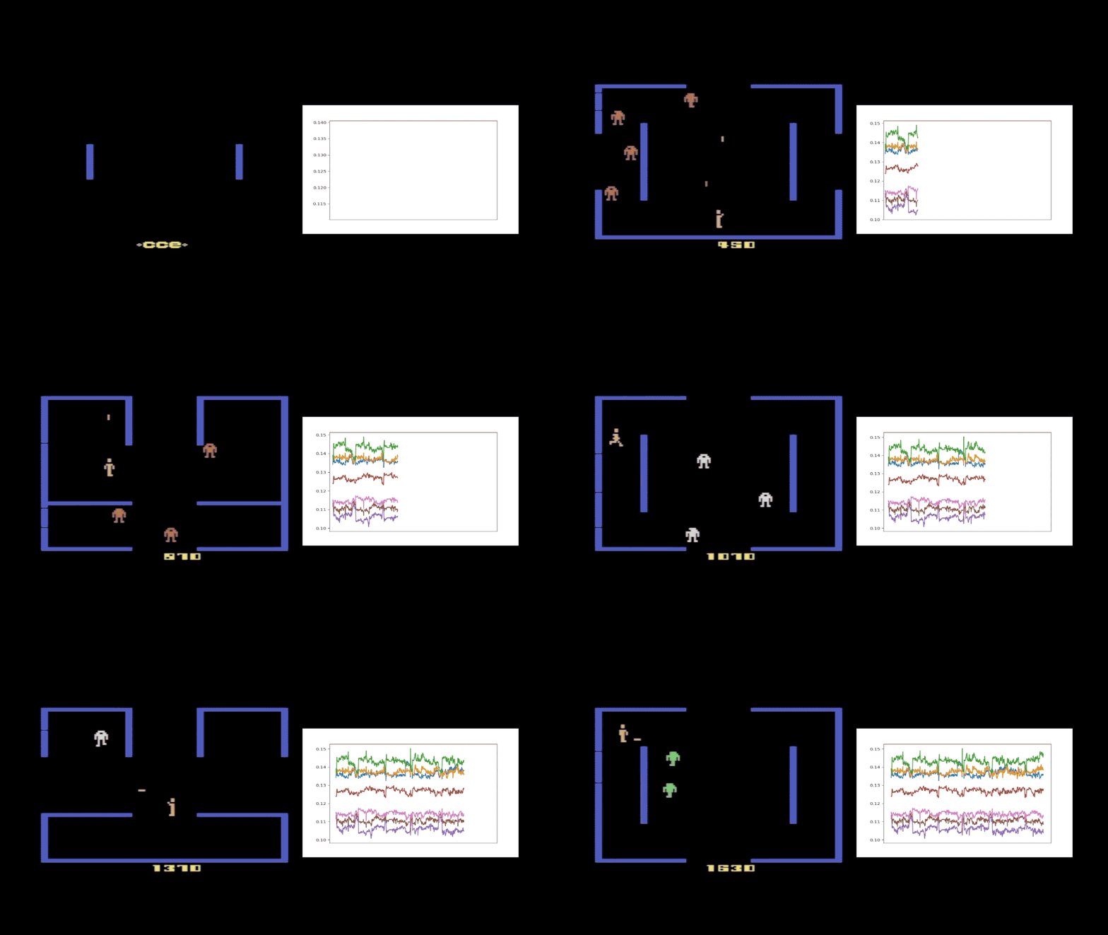
Figure 4: A half-trained Kung-Fu Master agent with eight probabilities, or quantile fractions, was selected to provide a case study of FQF. This figure shows how the interval between proposed quantile fractions varies during a single run. The different colors refer to different adjacent fractions’ intervals. Whenever an enemy appears behind the character, the fraction interval spikes, indicating the proposed fraction is very different from that of following states without enemies. This suggests that the fraction proposal network is state dependent and able to provide different quantile fractions accordingly.


