
From BiT (928 million parameters) to GPT-3 (175 billion parameters), state-of-the-art machine learning models are rapidly growing in size. With the greater expressivity and easier trainability of these models come skyrocketing training costs, deployment difficulties, and even climate impact. As a result, we’re witnessing exciting and emerging research into compressing these models to make them less expensive, small enough to store on any device, and more energy efficient. Perhaps the most popular approach to model compression is pruning, in which redundant model parameters are removed, leaving only a small subset of parameters, or a subnetwork. A major drawback of pruning, though, is it requires training a large model first, which is expensive and resource intensive.
Recent research around pruning has focused on the lottery ticket hypothesis (opens in new tab), which suggests that most parameters of large models are redundant even during training and that there exists a subnetwork responsible for most of the model’s performance. In other words, you can train this subnetwork alone and still obtain the same accuracy as if you had trained all the parameters—provided you are able to identify the subnetwork first. While such subnetworks—called lottery tickets—have been shown to exist by pruning large networks after training, intensive efforts to design methods that guess them before training, such as GraSP (opens in new tab)and hybrid tickets (opens in new tab), haven’t achieved the same performance.
Are sparsity-based methods such as pruning and guessing lottery tickets the right way to obtain compressed models? As part of our paper “Initialization and Regularization of Factorized Neural Layers (opens in new tab),” which we’re presenting at the International Conference on Learning Representations (opens in new tab) (ICLR 2021), we revisit the alternative compression approach of factorized neural layers (opens in new tab). While sparsity-based approaches remove parameters from the weight matrices of a network incrementally, factorization replaces the matrices with products of smaller matrices that are more efficient to store and compute. Despite the fact that factorized layers are more amenable to deployment on deep learning accelerators such as GPUs and software frameworks such as PyTorch, sparsity-based methods remain more popular because they’re seen as better at maintaining high accuracy at high compression rates (opens in new tab) (for example, 10 percent or less parameters remaining).
Microsoft Research Blog
Microsoft Research Forum Episode 3: Globally inclusive and equitable AI, new use cases for AI, and more
In the latest episode of Microsoft Research Forum, researchers explored the importance of globally inclusive and equitable AI, shared updates on AutoGen and MatterGen, presented novel use cases for AI, including industrial applications and the potential of multimodal models to improve assistive technologies.
Our results contradict this position: we show that if we use the right initialization scheme (spectral initialization, or SI) and the right regularization penalty (Frobenius decay, or FD), we can achieve higher accuracy on three benchmark datasets by training a factorized ResNet from scratch than by pruning or guessing lottery tickets. The key principle underlying these two natural methods, neither of which requires extra hyperparameters, is that the training behavior of a factorized model should mimic that of the original (unfactorized) network.
We further demonstrate the usefulness of these schemes in two settings beyond model compression where factorized neural layers are applied. The first is an exciting new area of knowledge distillation in which an overcomplete factorization is used to replace the complicated and expensive student-teacher training phase with a single matrix multiplication at each layer. The second is for training Transformer-based architectures such as BERT (opens in new tab), which are popular models for learning over sequences like text and genomic data and whose multi-head self-attention mechanisms are also factorized neural layers.
Our work is part of Microsoft Research New England’s (opens in new tab) AutoML research efforts (opens in new tab), which seek to make the exploration and deployment of state-of-the-art machine learning easier through the development of models that help automate the complex processes involved. The code to our work is available at our GitHub repository (opens in new tab).
Factorized neural layers and where to find them
Deep networks are function approximators in which inputs are passed through a sequence of nonlinear transformations \(g(W,x)\), each modifying the previous layer’s output \(x\) using some mapping specified by a weight matrix \(W\)∈ \(\mathbb{R}\)\(^m\)\(^x\)\(^n\). The space and time complexity of each layer is typically tied directly to the dimensionality of this weight matrix; for example, standard implementations of fully connected and convolutional layers require \(O(mn)\) operations to compute \(g(W, x)\).
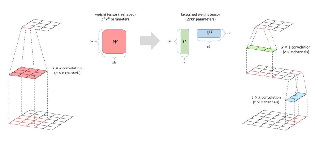
Factorized neural layers replace the matrix with a product of matrices; in the simplest case, we have the standard low-rank decomposition \(W\)=\(UV\)\(^T\) for matrices \(U\)∈ \(\mathbb{R}\)\(^m\)\(^x\)\(^r\), \(V\)∈ \(\mathbb{R}\)\(^n\)\(^x\)\(^r\). In the model compression case, we can set \(r\)≪\(m,n\) to improve the complexity of fully connected and convolutional layers from \(O(mn)\) to \(O(r(m+n))\); as shown in Figure 1, for two-dimensional convolutions, this speedup is achieved using two one-dimensional convolutions, one along each spatial dimension. In the case of Transformers, which take as input a sequence \(x\) with hidden dimension \(d\), we can express the action of a multi-head attention (MHA) operation parameterized by \(H\) query \((Q_h)\), key \((K_h)\), value \((V_h)\), and output \((O_h)\) projection matrices as the following summation over its heads \(h\)=1,…,\(H\):

This formulation makes clear that MHA is an aggregation over \(2H\) factorized neural layers with rank \(r=d/H\), half of them parameterized by \(Q_h\) \(Kh^T\) and the other half by \(V_h\) \(O_h^T\).
How should training routines handle factorized neural layers?
It’s straightforward to apply standard deep network training algorithms such as stochastic gradient descent (SGD) to networks with factorized layers. However, modern optimization procedures have many critical aspects, such as initialization and regularization, that significantly influence the performance of the final model. When we factorize a network, the effect of these components can change substantially, so we often can’t use the same settings as for the unfactorized model. For example, in the unfactorized case, the standard weight decay regularization penalizes the squared Frobenius norm (opens in new tab) ||\(W||_{Fro}^{2}\) of each weight matrix in the model; however, if we directly apply this to the factors \(U\) and \(V\) in a factorized layer, we end up penalizing an upper bound on twice the nuclear norm (opens in new tab) of their product:

As indicated in the figure below, this upper bound is tight when training a factorized ResNet using regular weight decay, showing that it effectively penalizes the nuclear norm rather than the Frobenius norm.
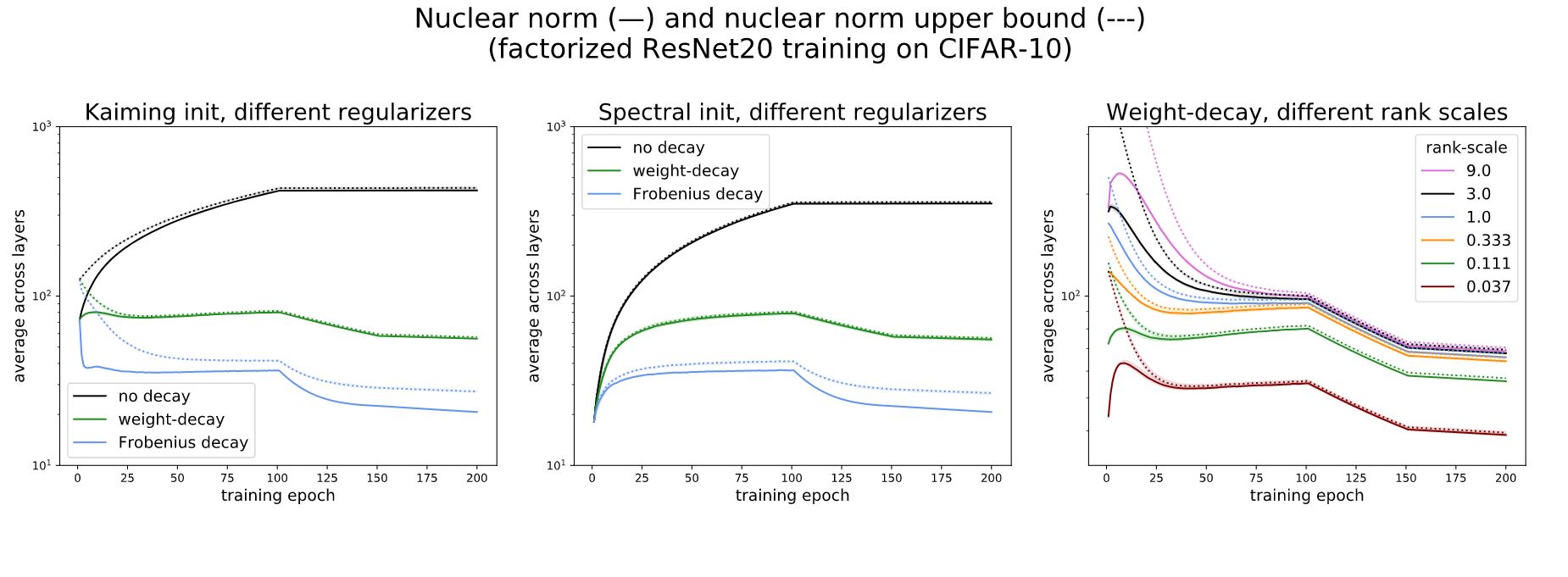
This example demonstrates how factorizing the model without modifying the training routine can lead to substantial changes in training behavior. Thus, following the principle that the training behavior of a factorized model should mimic that of the original model to recover the latter’s performance, we argue in favor of using spectral initialization (SI) and Frobenius decay (FD) when training factorized neural layers. SI initializes \(U\) and \(V\) by applying a rank-deficient singular value decomposition (SVD) to the standard random initialization of the corresponding full-rank weight matrix \(W\) in the original model, while FD replaces weight decay by penalizing the squared Frobenius norm ‖\(UV\)\(^T\)‖\(_{Fro}^{2}\) rather than the sum of squared norms of the individual factors.
In our paper, we extend a recent approximate analysis of weight decay (opens in new tab) to show that these two schemes allow SGD to maintain a high effective step size when training factorized neural layers, mimicking the role of regular weight decay applied to the original models. More informally, SI follows the mimicking principle since the SVD provably returns the best factorized approximation of initialization used by the original model. FD follows the mimicking principle by regularizing the squared Frobenius norm of the product, as is done by weight decay applied to the original model; in contrast, applying weight decay to the individual factors implicitly regularizes the nuclear norm, as shown in the figure above. Together, these two simple, efficient modifications lead to substantial improvements in model compression, knowledge distillation, and the training of Transformer-based architectures.
Factorization vs. sparsity-based methods for model compression
As mentioned above, sparsity-based approaches such as pruning and guessing lottery tickets represent the prevailing trend in model compression. However, in this section, we show that low-rank factorization is competitive with these methods and can even attain better accuracy at the same parameter count. In particular, the figure below demonstrates that, in the case of low-memory ResNets, factorized neural layers outperform not only sparse (low-memory) training methods like guessing lottery tickets and dynamic sparsity (opens in new tab) but often even full model training followed by pruning. The model—a modified ResNet32—and datasets—CIFAR-10, CIFAR-100, and Tiny-ImageNet—we use reflect the same standard setup considered by the lottery ticket papers GraSP and hybrid tickets.

This superior performance depends critically on the use of spectral initialization and Frobenius decay in tandem; interestingly, in the paper, we find that both schemes decrease accuracy when used independently. While factorization isn’t always best at very high compression rates, the figure above shows that it’s clearly superior in the standard lottery ticket regime, when the compressed model accuracy is close to that of the original model (usually this means the compressed model has 10 percent or more of the original parameters). Notably, our approach doesn’t require any additional tuning, as the decay coefficient used for the uncompressed model is the same one used by FD. Thus, factorized neural layers serve as a strong, simple baseline regardless of whether we’re targeting memory savings or fast computation.
Teacher-free teaching with overcomplete knowledge distillation
While our motivating application is model compression, factorized neural layers can also be found in other applications, such as knowledge distillation, a field that studies how to obtain a better small model by “teaching” it using a more powerful large model. Recent work on using overparameterization to train compact networks (opens in new tab) suggests that factorized neural layers can help us avoid the (expensive) two-stage student-teacher training process of knowledge distillation by using an overcomplete factorization of each of the student’s weight matrices \(W\)=\(UV\)\(^T\), where matrix factors \(U\)∈ \(\mathbb{R}\)\(^m\)\(^x\)\(^r\),\(V\)∈ \(\mathbb{R}\)\(^n\)\(^x\)\(^r\) have inner dimension \(r\)≥\(m,n\), making the factors wider than the original weight matrix, or even by using a deep factorization \(W\)=\(UMV\)\(^T\). The goal is to take advantage of the training benefits of deeper or wider networks suggested by recent theoretical work (opens in new tab) while not actually increasing the model capacity. While this increases the parameter count during training, afterward we can directly obtain a network of the original size by multiplying the factors together. We refer to this technique as overcomplete knowledge distillation.
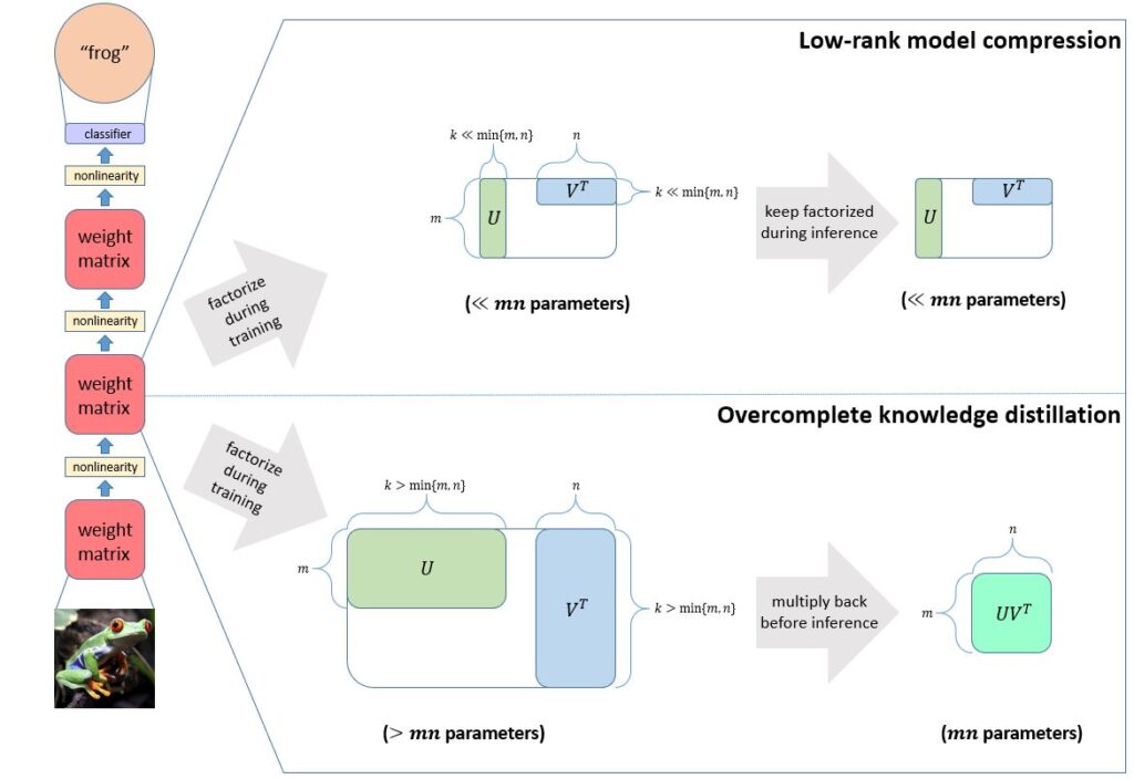
Since spectral initialization isn’t applicable when the decomposition is overcomplete, we investigate the effect of Frobenius decay alone. We find that this regularization is critical for overcomplete knowledge distillation using ResNets trained on CIFAR data; in fact, overparameterizing and applying regular weight decay decreases model accuracy. On the other hand, using FD, we can train an overparameterized ResNet56 (1.7 million parameters during training/850,000 parameters at inference time) that matches the performance of ResNet110 (1.7 million parameters at both training and inference). Furthermore, training the overcomplete ResNet56 is 1.5 times faster than training the regular ResNet110. These results are the first successful application of overcomplete knowledge distillation for large-depth neural networks on CIFAR.
Factorization-aware training of Transformers
Finally, we apply spectral initialization and Frobenius decay in the MHA module of Transformer-based architectures. While we can show that this indeed helps when training such models using regular SGD, large-scale unsupervised models, such as BERT, are usually trained using variants of adaptive algorithms such as Adam (opens in new tab)or LAMB (opens in new tab)that “decouple (opens in new tab)” weight decay by defining it as an operation that subtracts a small constant times the parameter from itself before taking a gradient step. While the equivalence breaks for adaptive methods, in the case of SGD, this is equivalent to adding a squared Frobenius penalty term to the objective. Thus for adaptive algorithms, we can devise a similar “decoupled” FD scheme that subtracts a small constant times \(UV\)\(^T\) \(V\)=∇\(_U\)\(_{2}^{1/}\) ‖\(UV\)\(^T\) ‖ \(_{Fro}^{2}\) and \(VU\)\(^T\) \(U\)=∇\(_V\)\(_{2}^{1/}\) ‖\(UV\)\(^T\) ‖\(_{Fro}^{2}\) from the factors \(U\) and \(V\), respectively.
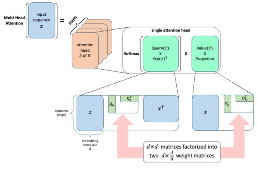
Applying FD in this manner to the MHA module when pretraining BERT-Base (110 million parameters) on unsupervised data yields a better downstream evaluation on the SQuAD task. When the MHA embedding dimension is halved (14.3 million fewer parameters), the advantage of FD continues to hold. On BERT-Large (340 million parameters), we’re able to halve the MHA embedding dimension (44.2 million fewer parameters) while losing less than a point in terms of F1-score.
Next steps in efficient model training
By studying how a standard initialization scheme and standard regularization scheme need to be modified to handle factorized layers, we were able to obtain better algorithms for learning efficient models, knowledge distillation, and training Transformers. We hope these results spur more investigation into how different components of standard training pipelines behave when training efficient models from scratch. For example:
- How should techniques like Dropout and BatchNorm be modified for factorized layers?
- Can we improve performance by factorizing using SVD after a few epochs of unfactorized model training rather than upon initialization (opens in new tab)?
- What aspects of model training should be changed when leveraging sparse or tensorial methods?
- Are different models better suited to different compression schemes?
| Virtual speaker series |
| Would you like to know more about AutoML research and its community at Microsoft? Join us for our free virtual speaker series “Directions in ML: AutoML and Automating Algorithms.” Learn more and register. |
We’re excited by how this work can advance cost-effective, high-performing models capable of running on any device. We’re also exploring the link between training compute time and energy consumption. Compute power for model training has been doubling at a rapid pace (opens in new tab). By reducing the required training time, our method for directly training smaller models raises the possibility of reducing energy consumption, as well. To learn more about the connections between compute and model architectures and power demands, check out the panel “Frontiers in Machine Learning: Climate Impact of Machine Learning (opens in new tab).”
Acknowledgments
This work was led by Carnegie Mellon University PhD student Misha Khodak, in collaboration with Neil Tenenholtz, Lester Mackey, and Nicolò Fusi, during a Microsoft Research internship.


