Dynamical systems theory provides a mathematical framework for studying how complex systems evolve over time, such as the neurons in our brains, the global climate system, or engineered cells. But predicting how these systems will behave in the future or how they might respond to disruption requires an accurate model.
Even writing down a model structure is complicated by the fact that the components of complex systems are often poorly understood or unknown. One must also determine the values of parameters that quantify how these components influence one another. By collecting measurements of the system over time, machine learning methods can be used to train a model that provides the predictions needed to accelerate science and engineering of complex systems.
Spotlight: Event Series
In a paper presented at the International Conference on Machine Learning (ICML) (opens in new tab), our team of researchers at Microsoft Research, led by Intern Geoffrey Roeder, Principal Scientist Neil Dalchau, and Principal Researcher Ted Meeds, developed a method that brings modern approaches from machine learning to efficiently parameterize both prescribed (white-box) and neural (black-box) dynamical systems models. This research is closely associated with the Station B project (opens in new tab), which you can learn more about on episode 67 of the Microsoft Research Podcast (opens in new tab) and in this story (opens in new tab).
Now, we have released the Python code and data from our research on GitHub (opens in new tab), which will allow others to reproduce our work and apply it to other scenarios to make further advancements using the technology.
Challenge #1: Using variational autoencoders (VAEs) for hierarchical parameters
One of the principle factors that makes parameter inference challenging in this context is that measurements are often collected for a range of individuals (such as molecules, cells, or patients), which may each exhibit slightly different behaviors in response to changing external conditions. Therefore, some model parameters might be “nuisance” parameters that need to be assigned a different value for each individual. We refer to these as individual-level parameters.
In addition, individuals can often be grouped by specific characteristics (such as by genotype) with group-level parameters that are assigned a different value for each group. Finally, there will also be global population parameters that are assigned the same value across individuals and groups, such as the binding affinities or degradation rates of specific molecules.
This hierarchical parameter space creates a problem for a naïve inference strategy that simply samples a subset of the parameter values, evaluates model performance, and then takes a step in the parameter space. Varying global parameters will affect all data points, while varying individual or group parameters will only affect specific data points relating to that individual or group. Therefore, more samples are needed to train these parameter values effectively.
Taking a Bayesian approach to inference provides several advantages over pure optimization, as it provides a statistical assessment of trained model variables and uncertainty measures for predictions. For example, if only a few measurements are available to train a model, then the learning process won’t significantly reduce uncertainty in a model prediction, whereas when more data is available, one can make more certain predictions.
When using pure optimization, no assessment can be made about the confidence of a prediction. However, it can be computationally costly to evaluate posterior distributions for large numbers of variables. Variational inference offers a computationally cheaper alternative, approximating the distributions of each variable by a Gaussian, which requires just two quantities (µ,σ2). This enables predictions to be made with approximated uncertainty estimates, retaining a major benefit of Bayesian inference.
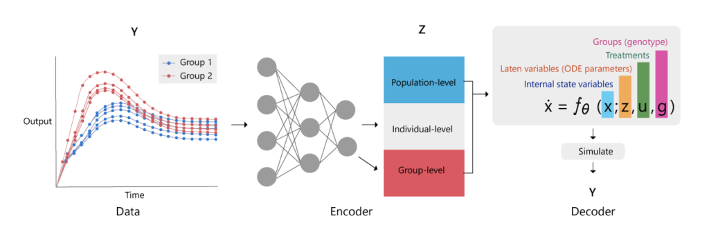
The recent advances in variational autoencoders (VAEs) are of specific relevance to our application. Encoders approximate the data space by a lower-dimensional representation in a latent space and can be trained as neural networks that take data as inputs and produce the desired latent space as an output (Figure 1).

(opens in new tab) Figure 1: Structure of a variational autoencoder for hierarchical dynamical systems. The goal is to approximate the posterior distributions of the ordinary differential equation variables z, which include population-level (blue), individual-level (black) and group-level (pink) variables. An encoder neural network is trained to convert observational data Y, inputs u, and group memberships g into the variational approximations (parameters μ and σ) for each variable z_j. By decoding these parameters via the ordinary differential equation model, we obtain a reconstruction of the data, which provides an objective for learning.
Here, the time-series data is encoded in a latent space represented by the mean and precision of each parameter in the model. This latent space is then decoded by simulating the model equations, therefore obtaining a simulation of the measured time-series outputs. The training of the model parameters proceeds by training neural network weights that encode the distributions of the model parameters from the data in an optimal way with respect to the decoder. An approximation of the marginal likelihood, the evidence lower bound (ELBO), is then used as an objective function by the ADAM optimizer, as implemented in TensorFlow (opens in new tab). This brings us to the second challenge.
Challenge #2: Using importance sampling and a modified Euler scheme for numerical integration
Obtaining simulations of differential equation models is cumbersome due to the need for numerical integration of the model equations. Additionally, to make use of gradient-based optimizers such as Adam, the full model simulation must be differentiable.
A variant of variational autoencoders is the importance-weighted autoencoder (IWAE), which is thought to learn richer latent space representations. An additional benefit of importance sampling in this context is that it enables the simultaneous evaluation of multiple samples, alleviating the need to form long Markov chains during inference.
We used a simple modified Euler scheme for numerical integration, which was sufficient for our case study and, crucially, could be implemented as a while loop in TensorFlow, enabling auto-differentiation of the ELBO. An obvious future improvement to this approach would be to use the adjoint method proposed in the NeurIPS 2019 (opens in new tab) paper, “Neural Ordinary Differential Equations (opens in new tab)” by Ricky T.Q. Chen and others, which enables arbitrary numerical integration libraries to be used alongside gradient-based optimization.
Challenge #3: Using neural ordinary differential equation models to tackle model misspecification
As mentioned above, it is often difficult to know the structure of a differential equation model for a complex system. Incorrectly specifying the model with respect to the real system can result in false predictions being made. Model misspecification can also introduce biases in parameter estimates, affecting insights on the functioning and quantitative properties of the system of interest.
We explored using neural ordinary differential equations, a black-box model class that was recently introduced in the paper (opens in new tab) mentioned above. We developed our framework to work seamlessly with both prescribed and black-box models (or a mixture of the two). In doing so, we showed how the prediction capabilities of trained neural ordinary differential equation models can significantly outperform prescribed models on real biological data.
To learn more about our synthetic biology case study and how our variational autoencoders facilitate efficient inference, please read our ICML paper (opens in new tab). The Python code and data can be found in a repository called VI-HDS (opens in new tab) (variational inference for hierarchical dynamical systems). The package is built using TensorFlow and benefits from TensorBoard visualizations during training. Again, we hope that providing the Python code and data will enable researchers to apply our research to other scenarios and make further advancements.


