A game-theoretic approach to provably correct and scalable offline RL

Despite increasingly widespread use of machine learning (ML) in all aspects of our lives, a broad class of scenarios still rely on automation designed by people, not artificial intelligence (AI). In real-world applications that involve making sequences of decisions with long-term consequences, from allocating beds in an intensive-care unit to controlling robots, decision-making strategies to this day are carefully crafted by experienced engineers. But what about reinforcement learning (RL), which gave machines supremacy in games as distinct as Ms. PacMan and Pokémon Go? For all its appeal, RL – specifically, its most famous flavor, online RL – has a significant drawback beyond scenarios that can be simulated and have well-defined behavioral rules. Online RL agents learn by trial and error. They need opportunities to try various actions, observe their consequences, and improve as a result. Making wildly suboptimal decisions just for learning’s sake is acceptable when the biggest stake is a premature demise of a computer game character or showing an irrelevant ad to a website visitor. For tasks such as training a self-driving car’s AI, however, it is clearly not an option.

Offline reinforcement learning (RL) is a paradigm for designing agents that can learn from large existing datasets – possibly collected by recording data from existing reliable but suboptimal human-designed strategies – to make sequential decisions. Unlike the conventional online RL, offline RL can learn policies without collecting online data and even without interacting with a simulator. Moreover, since offline RL does not blindly mimic the behaviors seen in data, like imitation learning (an alternate strategy of RL), offline RL does not require expensive expert-quality decision examples, and the learned policy of offline RL can potentially outperform the best data-collection policy. This means, for example, an offline RL agent in principle can learn a competitive driving policy from logged datasets of regular driving behaviors. Therefore, offline RL offers great potential for large-scale deployment and real-world problem solving.

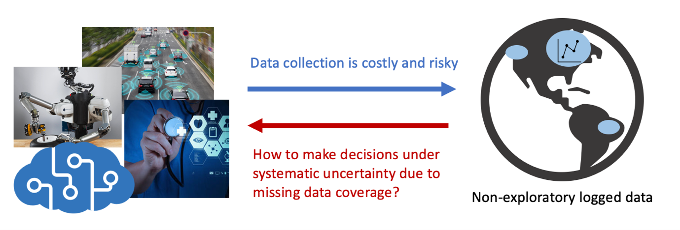
However, offline RL faces a fundamental challenge: the data we can collect in large quantity lacks diversity, so it is impossible to use it to estimate how well a policy would perform in the real world. While we often associate the term “Big Data” with diverse datasets in ML, it is no longer true when the data concerns real-world “sequential” decision making. In fact, curating diverse datasets for these problems can range from difficult to nearly impossible, because it would require running unacceptable experiments in extreme scenarios (like staging the moments just before a car cash, or conducting unethical clinical trials). As a result, the data that gets collected in large quantity, counterintuitively, lacks diversity, which limits its usefulness.

In this post, we introduce a generic game-theoretic framework for offline RL. We frame the offline RL problem as a two-player game where a learning agent competes with an adversary that simulates the uncertain decision outcomes due to missing data coverage. By this game analogy, we design a systematic and provably correct way to design offline RL algorithms that can learn good policies with state-of-the-art empirical performance. Finally, we show that this framework provides a natural connection between offline RL and imitation learning through the lens of generative adversarial networks (GANs). This connection ensures that the policies learned by this game-theoretic framework are always guaranteed to be no worse than the data collection policies. In other words, with this framework, we can use existing data to robustly learn policies that improve upon the human-designed strategies currently running in the system.

The content of this post is based on our recent papers Bellman-consistent Pessimism for Offline Reinforcement Learning (Oral Presentation, NeurIPS 2021) and Adversarially Trained Actor Critic for Offline Reinforcement Learning (Outstanding Paper Runner-up, ICML 2022).

Fundamental difficulty of offline RL and version space

A major limitation of making decisions with only offline data is that existing datasets do not include all possible scenarios in the real world. Hypothetically, suppose that we have a large dataset of how doctors treated patients in the past 50 years, and we want to design an AI agent to make treatment recommendations through RL. If we run a typical RL algorithm on this dataset, the agent might come up with absurd treatments, such as treating a patient with pneumonia through amputation. This is because the dataset does not have examples of what would happen to pneumonia after amputating patients, and “amputation cures pneumonia” may seem to be a plausible scenario to the learning agent, as no information in the data would falsify such a hypothesis.

To address this issue, the agent needs to carefully consider uncertainties due to missing data. Rather than fixating on a particular data-consistent outcome, the agent should be aware of different possibilities (i.e., while amputating the leg might cure the pneumonia, it also might not, since we do not have sufficient evidence for either scenario) before committing to a decision. Such deliberate conservative reasoning is especially important when the agent’s decisions can cause negative consequences in the real world.

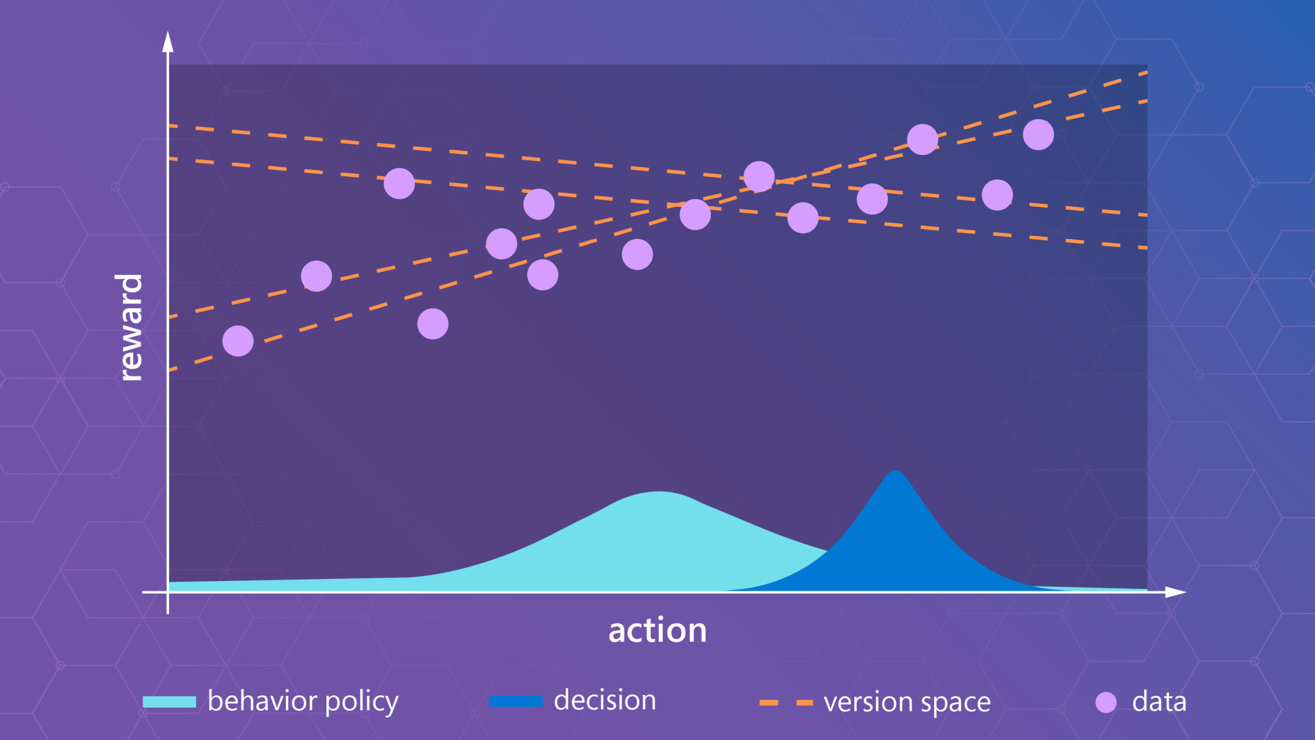
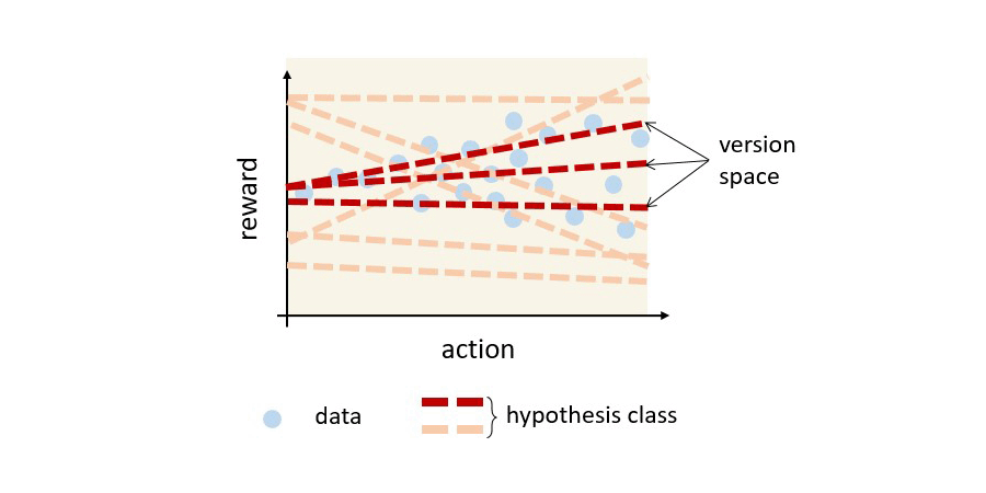
A formal way to express the idea above is through the concept of version space. In machine learning, a version space is a set of hypotheses consistent with data. In the context of offline RL, we will form a version space for each candidate decision, describing the possible outcomes if we are to make the decision. Notably, the version space may contain multiple possible outcomes for a candidate decision whose data is missing.

To understand better what a version space is, we use the figure below to visualize the version space of a simplified RL problem where the decision horizon is one. Here we want to select actions that can obtain the highest reward (such as deciding which drug treatment has the highest chance of curing a disease). Suppose we have data of action-reward pairs, and we want to reason about the reward obtained by taking an action. If the underlying reward function is linear, then we have a version space shown in red, which is a subset of (reward) hypotheses that are consistent with the data. In general, for a full RL problem, a version space can be more complicated than just reward functions, e.g., we would need to start thinking about hypotheses about world models or value functions. Nonetheless, similar concepts like the one shown in the figure below apply.

Thinking offline RL as two-player games

If we think about uncertainties as hypotheses in a version space, then a natural strategy of designing offline RL agents is to optimize for the worst-case scenario among all hypotheses in the version space. In this way, the agent would consider all scenarios in the version space as likely, avoiding making decisions following a delusional outcome.

Below we show that this approach of thinking about worst cases for offline RL can be elegantly described by a two-player game, called the Stackelberg game. To this end, let us first introduce some math notations and explain what a Stackelberg game is.

Notation We use \(π\) to denote a decision policy and use \(J(π)\) to denote the performance of \(π\) in the application environment. We use \(Π\) to denote the set of policies that the learning agent is considering, and we use \(\mathcal{H}\) to denote the set of all hypotheses. We also define a loss function \(\psi:Π × \mathcal{H}→[0, \infty)\) such that if \(\psi(π,H)\) is small, \(H\) is a data-consistent hypothesis with respect to \(π\); conversely \(\psi(π,H)\) gets larger for data-inconsistent ones (e.g., we can treat each \(H\) as a potential model of the world and \(\psi(π,H)\) as the modelling error on the data). Consequently, a version space above is defined as \(\mathcal V_\pi = \{ H: \psi(\pi,H) \leq \varepsilon \}\) for some small \(\varepsilon\).

Given a hypothesis \(H \in \mathcal{H}\), we use \(H(π)\) to denote the performance of \(π\) \(predicted\) by \(H\), which may be different from \(π\)’s true performance \(J(π)\). As a standard assumption, we suppose for every \(π \in Π\) there is some \(H_{π}^* \in \mathcal{H}\) that describes the true outcome of \(π\), that is, \(J(π) = H_{π}^*(π)\) and \(\psi(π,H_{π}^*) = 0\).

Stackelberg Game In short, a Stackelberg game (opens in new tab) is a bilevel optimization problem,

\(\displaystyle \max_{x} f(x,y_x), \quad {\rm s.t.} ~~ y_x \in \min_x g(x,y)\)

In this two-player game, the Leader \(x\) and the Follower \(y\) maximize and minimize the payoffs \(f\) and \(g\), respectively, under the rule that the Follower plays after the Leader. (This is reflected in the subscript of \(y_{x}\), that \(y\) is decided based on the value of \(x\)). In the special case of \(f = g\), a Stackelberg game reduces to a zero-sum game \(\displaystyle \max_{x} \min_{y} f(x,y)\).

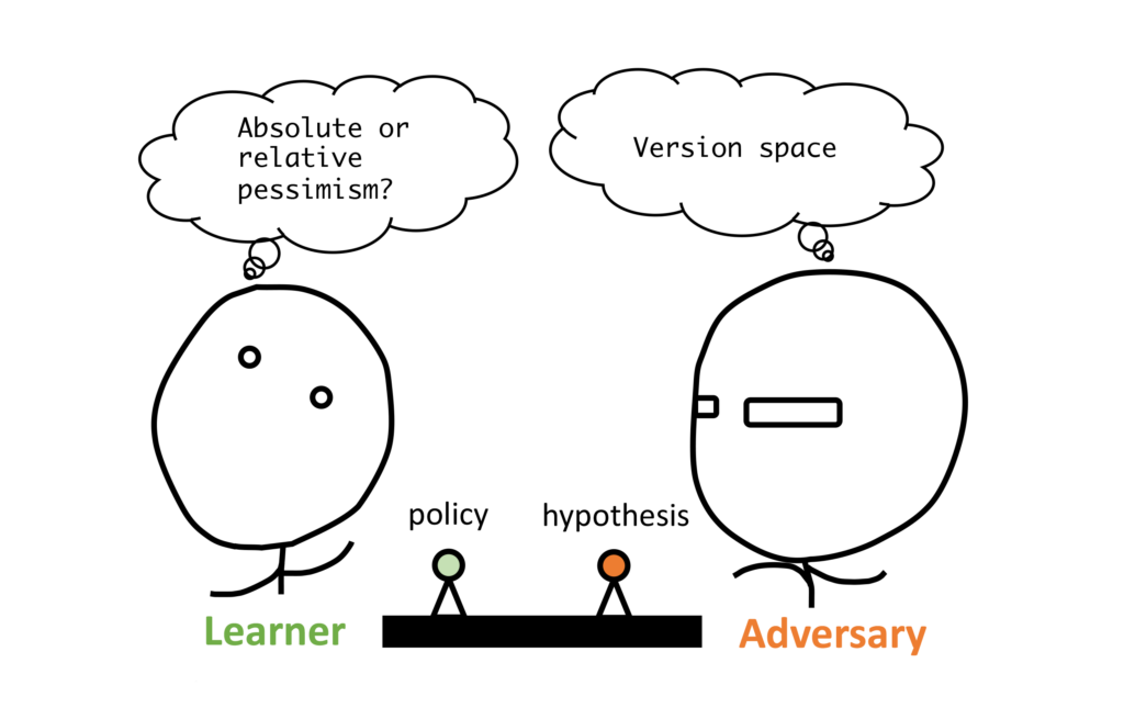
We can think about offline RL as a Stackelberg game: We let the learning agent be the Leader and introduce a fictitious adversary as the Follower, which chooses hypotheses from the version space \(V_{π}\) based on the Leader’s policy \(π\). Then we define the payoffs above as performance estimates of a policy in view of a hypothesis. By this construction, solving the Stackelberg would mean finding policies that maximize the worst-case performance, which is exactly our starting goal.

Now we give details on how this game can be designed, using absolute pessimism or relative pessimism, so that we can have performance guarantees in offline RL.

A two-player game based on absolute pessimism

Our first instantiation is a two-player game based on the concept of absolute pessimism, introduced in the paper Bellman-consistent Pessimism for Offline Reinforcement Learning (NeurIPS 2021).

\(\displaystyle \max_{\pi \in \Pi} H_\pi(\pi), \quad {\rm s.t.} ~~ H_\pi \in \min_{H \in \mathcal H} H(\pi) + \beta \psi(\pi,H) \)

where \(\beta \ge 0\) is a hyperparameter which controls how strongly we want the hypothesis to be data consistent. That is, the larger \(\beta\) is, the smaller the version space \(\mathcal V_\pi = \{ H: \psi(\pi,H) \leq \varepsilon \}\) is (since \(\varepsilon\) is smaller), so we can think that the value of \(\beta\) trades off conservatism and generalization in learning.

This two-player game aims to optimize for the worst-case absolute performance of the agent, as we can treat \(H_{π}\) as the most pessimistic hypothesis in \(\mathcal{H}\) that is data consistent. Specifically, we can show \(H_{π}(π) \le J(π)\) for any \(\beta \ge 0\); as a result, the learner is always optimizing for a performance lower bound.

In addition, we can show that by the design of \(\psi\), this lower bound is tight when \(\beta\) is chosen well (that is, it only underestimates the performance when the policy runs into situations for which we lack data). As a result, with a properly chosen \(\beta\) value, the policy found by the above game formulation is optimal, if the data covers relevant scenarios that an optimal policy would visit, even for data collected by a sub-optimal policy.

In practice, we can define the hypothesis space \(\mathcal{H}\) as a set of value critics (model-free) or world models (model-based). For example, if we set the hypothesis space \(\mathcal{H}\) as candidate Q-functions and \(\psi\) as the Bellman error of a Q function with respect to a policy, then we will get the actor-critic algorithm called PSPI (opens in new tab). If we set \(\mathcal{H}\) as candidate models and \(\psi\) as the model fitting error, then we get the CPPO (opens in new tab) algorithm.

A two-player game based on relative pessimism

While the above game formulation guarantees learning optimality for a well-tuned hyperparameter \(\beta\), the policy performance can be arbitrarily bad if the \(\beta\) value is off. To address this issue, we introduce an alternative two-player game based on relative pessimism, proposed in the paper Adversarially Trained Actor Critic for Offline Reinforcement Learning (ICML 2022).

\(\displaystyle \max_{\pi \in \Pi} H_\pi(\pi) \color{red}{- {H_{π}(\mu)}}, \ \ {\rm s.t.} \ \ H_{π} \in \min_{H \in \mathcal H} H(π) \color{red}{- {H(\mu)}} + \beta\psi(π,H)\)

where we use \(\mu\) to denote the data collection policy.

Unlike the absolute pessimism version above, this relative pessimism version is designed to optimize for the worst-case performance relative to the behavior policy \(\mu\). Specifically, we can show \(H_\pi (\pi) – H_\pi(\mu) \leq J(\pi) – J(\mu)\) for all \(\beta \ge 0\). And again, we can think about the hypotheses in model-free or model-based manners, like the discussion above. When instantiated model-free, we get the ATAC (Adversarially Trained Actor Critic) algorithm, which achieves state-of-the-art empirical results in offline RL benchmarks.

An important benefit of this relative pessimism version is a robust property to the choice of \(\beta\). As a result, we can guarantee that the learned policy is always no worse than the behavior policy, despite data uncertainty and the \(\beta\) choice – a property we call \(robust\) \(policy\) \(improvement\). The intuition behind this is that \(\pi = \mu\) achieves a zero objective in this game, so the agent has an incentive to deviate from \(\mu\) only if it finds a policy \(\pi\) that is uniformly better than \(\mu\) for all possible data-consistent hypotheses.

At the same time, this relative pessimism game is also guaranteed with the learning optimality when \(\beta\) is chosen correctly, just like above absolute pessimism game. Therefore, in some sense, we can view the relative pessimism game (e.g., ATAC) as a robust version of the absolute pessimism game (e.g., PSPI).

A connection between offline RL and imitation learning

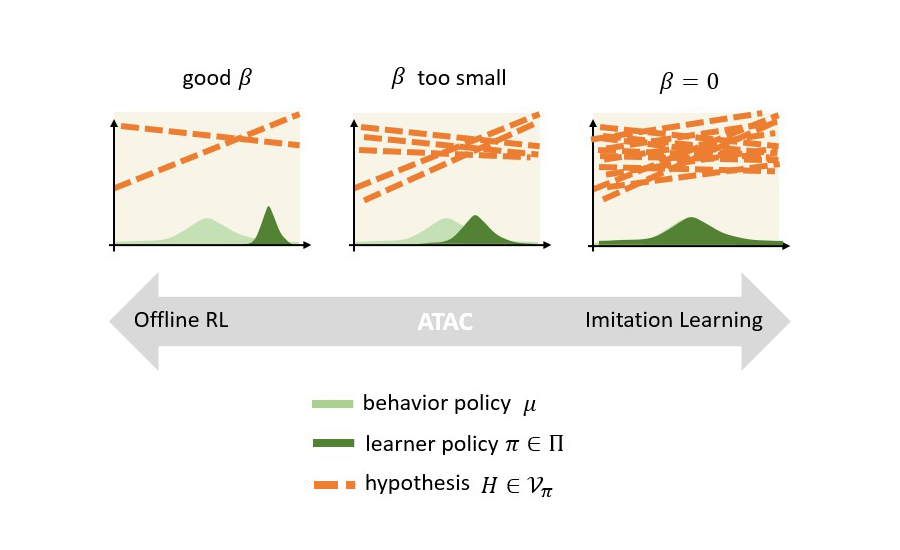
An interesting takeaway from the discussion above is a clean connection between offline RL and imitation learning (IL) based on GANs or integral probability metric. IL like offline RL also tries to learn good policies from offline data. But IL does not use reward information, so the best strategy for IL is to mimic the data collection policy. Among modern IL algorithms, one effective strategy is to use GANs, where we train the policy (the generator) using an adversarial discriminator to separate the actions generated the policy and the actions from the data.

Now that we understand how IL-based on GANs work, we can see the connection between offline RL and IL through the model-free version of the relative pessimism game, that is, ATAC. We can view the actor and the critic of ATAC as the generator and the discriminator in IL based on GANs. By choosing different \(\beta\) values, we can control the strength of the discriminator; when \(\beta = 0\), the discriminator is the strongest, and the best generator is naturally the behavior policy, which recovers the imitation learning behavior. On the other hand, using larger \(\beta\) weakens the discriminator by Bellman regularization (i.e., \(\psi\)) and leads to offline RL.

In conclusion, our game-theoretic framework shows

Offline RL + Relative Pessimism = IL + Bellman Regularization.

We can view them both as solving a version of GANs problems! The only difference is that offline RL uses more restricted discriminators that are consistent with the observed rewards, since the extra information added in offline RL compared with imitation learning is the reward labels.

The high-level takeaway from this connection is that the policies learned by offline RL with the relative pessimism game are guaranteed to be no worse than the data collection policy. In other words, we look forward to exploring possible applications that robustly improve upon existing human-designed strategies running in the system, by just using existing data despite the lack of data diversity.

Opens in a new tab