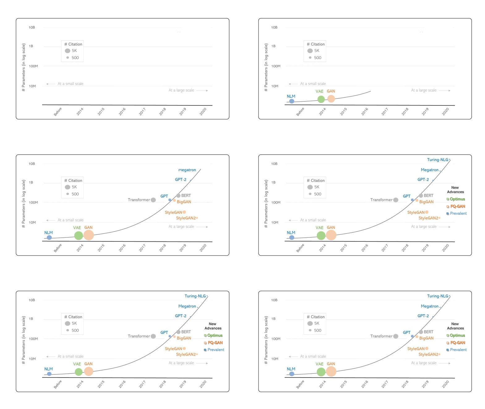
Figure 1: A brief evolution of deep generative models over time, measured by model size (number of parameters) and scientific impact (number of citations to date). Three popular deep generative model types are considered: Auto-regressive models (neural language models or NLMs) in blue, Variational Autoencoders (VAEs) in green, and Generative Adversarial Networks (GANs) in orange. Transformer and BERT are shown as references. The three new generative models we introduce in this post expand large-scale capabilities in each of these categories (right side of chart).
One of the core aspirations in artificial intelligence is to develop algorithms and techniques that endow computers with an ability to synthesize the observed data in our world. Every time researchers build a model to imitate this ability, this model is called a generative model. If deep neural networks are involved in this model, the model is a deep generative model (DGM). As a branch of self-supervised learning techniques in deep learning, DGMs specifically focus on characterizing data generation processes.
This post describes three projects that share a common theme: improving or applying DGMs in the era of large-scale datasets and training. In this post, we’ll first review the evolution history of DGMs, then introduce new advances in DGMs made by researchers from Microsoft Research, in collaboration with members from the University at Buffalo (opens in new tab) and Duke University (opens in new tab). The generative models presented here, and detailed in their corresponding papers, each fall into a different category of popular deep generative model. Optimus is the first large-scale Variational Autoencoder (opens in new tab) (VAE) language model, showing the opportunity of DGMs following a trend of pre-trained language models. FQ-GAN resolves scalability issues with image generation in Generative Adversarial Networks (opens in new tab) (GANs). Finally, we introduce Prevalent, the first pre-trained generic agent for vision-and-language navigation (opens in new tab). Let’s look at a quick overview of DGMs before diving into our new achievements.
Three types of generative models and a shared trick
Spotlight: Event Series
Generative models (opens in new tab) have a long history in traditional machine learning, and they are often distinguished from the other main approach, discriminative models (opens in new tab). One may learn how they differ from a story of two siblings (opens in new tab). In the story, the siblings have different special abilities: one has the ability to learn everything in great depth, while the other can only learn the differences between what he sees. These siblings represent a generative model, which characterizes actual distributions with an internal mechanism, and a discriminative model, which builds decision boundaries between classes.
With the rise of deep learning, a new family of methods, called deep generative models (DGMs), is formed through the combination of generative models and deep neural networks. Because neural networks used as generative models have a number of parameters smaller than the amount of data they are trained on, there is a trick that DGMs can perform. In an excellent blog post from OpenAI (opens in new tab), this trick is revealed: “…models are forced to discover and efficiently internalize the essence of the data in order to generate it.” To learn more about DGMs, check out recent lectures at Stanford University (opens in new tab), University of California Berkeley (opens in new tab), Columbia University (opens in new tab) and New York University (opens in new tab).
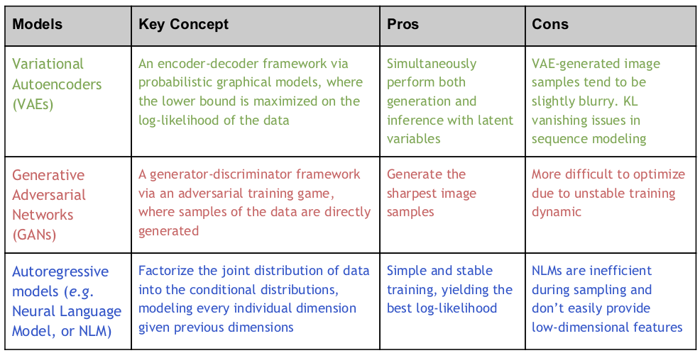
Mathematically, for a dataset of examples {\(x_{i}\)|\(x_{i}\) \( \in \) \(\mathbb{R}\)<sup><em>D</em></sup>, \(i\) = 1, … , \(N\)} as samples from a true data distribution \( q(x)\), the goal of a DGM is to build deep neural networks with parameters \(\theta\) \( \in \) \(\mathbb{R}\)<sup><em>P</em></sup>, to describe a distribution \(p_\theta\left(x\right) \) so that the parameters \(\theta\) can be trained to ensure \(p_\theta\left(x\right) \) match \(q(x)\) the best. All DGMs share this same basic setup and the above DGM trick, but they differ in the ways they approach the problem. There are three popular model types according to OpenAI taxonomy (opens in new tab): VAEs, GANs, and auto-regressive models. Each of these is detailed in the following table:
Moving from small-scale to large-scale deep generative models in all three categories
Thanks to many efforts on developing their theoretical principles over the years, DGMs are now relatively well understood at a small scale. The DGM trick mentioned above promises that the models work fine under a mild condition: \(P\)< \(N\)*\(D\). This has been verified in many early works at a small scale. However, recent years have witnessed tremendous advances and strong empirical results through pre-training large models on massive data (in the context of the equation above,\(N\)is increased dramatically).
Researchers from OpenAI believe that generative models are one of the most promising approaches to potentially reach the goal of endowing computers with an understanding of our world. Along these lines, they developed Generative Pre-training (opens in new tab) (GPT) in 2018, an autoregressive neural language model (opens in new tab) (NLM) trained on a diverse corpus of unlabeled text, followed by discriminative fine-tuning on each specific task, showing significantly improved performance on multiple language understanding tasks. In 2019, they further scaled this idea up to 1.5 billion parameters and developed GPT-2 (opens in new tab), which shows near-human performance in language generation. With more compute, Megatron (opens in new tab) and Turing-NLG (opens in new tab) inherit the same idea, and scale it up to 8.3 billion and 17 billion, respectively.
The above line of research shows that NLM has gained tremendous progress (\(P\) is increased dramatically in the equation above). Nevertheless, as an autoregressive model, NLM is just one of three types of DGMs. There are still two other types of DGMs (VAE and GAN) that can be significantly improved for large-scale uses. In this exciting era, large models are trained on large datasets with massive computing, which has given rise to a new learning paradigm: self-supervised pre-training with task-specific fine-tuning. DGMs have been studied less in this setting, and we are not sure if the tricks of DGMs can still work well in this setting for industrial practice. It raises a series of research questions, which we’ll explore in relation to each project below:
- Opportunity: How good are DGMs really with pre-training?
- Challenge: Are modifications required to make existing methods work in this setting?
- Application: Can DGMs benefit pre-training in contrast?
Optimus: Opportunities in language modeling
The central question addressed in this paper, called “Optimus: Organizing sentences via Pre-trained Modeling of a Latent Space, (opens in new tab)” is: What will happen if we scale up a VAE and use it as a new pre-trained language model (PLM)? To address this question, we created Optimus (Organizing sentences with pre-trained modeling of a universal latent space), the first large-scale deep latent variable model for natural language, which is pre-trained using the sentence-level (variational) autoencoder objectives on a large text corpus.
Pre-trained language models have made substantial advancements across a variety of natural language processing tasks. PLMs are often trained to predict words based on their context in massive text data, and the learned models can be fine-tuned to adapt to various downstream tasks. PLMs can generally play two different roles: a generic encoder such as BERT (opens in new tab) and Roberta (opens in new tab), and a powerful decoder such as GPT-2 (opens in new tab)and Megatron (opens in new tab). Sometimes, both tasks can be performed in one unified framework, such as in UniLM (opens in new tab), BART (opens in new tab), and T5 (opens in new tab). These models lack explicit modeling of structures in a compact latent space, rendering it difficult to control natural language generation and representation from sentence-level semantics.
When trained effectively, the Variational Autoencoder (VAE) (opens in new tab) can be both a powerful generative model and an effective representation learning framework for natural language. By representing sentences in a low-dimensional latent space, VAEs allow easy manipulation of sentences using the corresponding compact vector representations (like the smooth feature regularization specified by prior distributions) and guided sentence generation with interpretable latent vector operators. Despite the attractive theoretical strengths, the current language VAEs are often built with shallow network architectures, such as two-layer LSTMs (opens in new tab). This limits the model’s capacity and leads to suboptimal performance. When a large amount of data is given, the tricks of DGM may break if shallow VAE is employed.

For a sentence of length \(T\), \(x\) = \([x_{i}…,x_{T}]\), an autoregressive NLM generates current token \(x_{t}\) conditioned on the previous word tokens \( x\)<sub><\(t\)</sub>, as shown in Equation 1 above, there is limited capacity for the generation to be guided by the higher-level semantics. GPT-2 is perhaps the most well-known NLM instance, pre-trained on large amounts of text. In contrast, VAE generates \(x_{t}\) conditioned both previous word tokens \( x\)<sub><\(t\)</sub> and a latent variable \(z\), as shown in Equation 2 above. The latent \(z\) determines the high-level semantics (that is, the “outline”) of a sentence, such as tense, topics or sentiment, guiding a sequential decoding process to fill in details of the outline. The decoder \(\theta\) is combined with an encoder \(\phi\). VAEs learn the parameters by maximizing a lower bound (opens in new tab) on the log likelihood of the data.
![Figure 2a: Optimus Architecture,variable x moves through an encoder (made up pf BERT and H[CLS]) then moves through variable Z, then into a decoder (made up of variable H and GPT-2), and finally into variable x. Figure 2b: Memory: variable Z moves into a 3 by 4 square memory block. the first column of 3 squares is white. The rest are blue. Under the first blue column, X0, the second XT minus 1, the third X with subscript T. Embedding: variable Z moves through Latent plus Word plus Positional.](https://www.microsoft.com/en-us/research/uploads/prod/2020/04/Generative-Models-Fig-2-300x152.png)
Figure 2: (a) Optimus architecture, made up of an encoder and a decoder, and (b) latent vector injection.
- Language Modeling—We consider four datasets, including Penn Treebank (opens in new tab), SNLI (opens in new tab), Yahoo (opens in new tab), and Yelp (opens in new tab) corpora, and fine-tune the PLM for one epoch (opens in new tab) on each. Optimus achieves lower perplexity than GPT-2 on three of the four datasets, due to the knowledge encoded in the latent prior distribution. Compared with all existing small VAEs, Optimus shows much better representation learning performance, measured by mutual information (opens in new tab) and active units (opens in new tab). This implies that pre-training by itself is an effective approach to alleviate the KL vanishing issue.
- Guided Language Generation—Thanks to the latent variable, Optimus has the unique advantage to control sentence generation from a semantic level (GPT-2 is infeasible for this). It provides new ways one can play with language generation. In Figure 3 (below), we illustrate the idea using some simple latent vector manipulation in two scenarios: 1) sentence-level transfer via the arithmetic operation of latent vectors: \(z_{\tau}\) = \(z_{1}\) * (1 – \(\tau\)) + \(z_{2}\) * \(\tau\) and 2) sentence interpolation: \(z_{D}\) = \(z_{B}\) – \(z_{A}\) + \(z_{C}\), where \(\tau\) \(\in\) [0,1]. For more sophisticated latent space manipulation, we consider dialog response generation, stylized response generation, and label-conditional sentence generation. Optimus shows superiority to existing methods on all these tasks.
- Low-resource Language Understanding—Optimus learns a smoother space and more separated feature patterns than BERT (Figure 4a and 4b below). This allows Optimus to yield better classification performance and faster adaptation than BERT when used as a feature-based approach (the backbone network is frozen and only the classifier is updated), as it allows Optimus to maintain and exploit the latent structure learned in pre-training. Figure 4c shows the results with a varying number of labelled samples per class on this Yelp review dataset, Optimus shows much better results in the low-compute scenarios (feature-based settings). A similar comparison is observed on the GLUE benchmark.
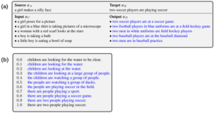
Figure 3: (a) sentence transfer; (b) sentence interpolation. Blue indicates generated sentences.

Figure 4: (a) and (b) Feature space visualization using tSNE for Optimus and BERT, respectively. Sentences with different labels are rendered in different colors. (c) Results with varying labelled data
Please check out our paper (opens in new tab) for more results, and play with Optimus on Github (opens in new tab)
FQ-GAN: Challenges in image generation
GAN is a popular model for image generation. It consists of two networks—a generator to directly synthesize fake samples that mimic real samples and a discriminator to distinguish between real samples \((x)\) and fake samples \((\hat{x})\). The two networks are trained in an adversarial manner so that the fake data distribution can match the real data distribution.
Feature matching (opens in new tab) is a principled technique that casts the data distribution matching problem of GANs into a distribution matching problem in the feature space of the discriminator. This requires feature statistics (first or second order moments), estimated from the entirety of both fake and real samples, to be similar. In practice, these feature statistics are estimated using mini-batches in a continuous feature space. As the dataset becomes much larger and more complex (for example, higher resolutions), the quality of mini-batch based estimate becomes poor because the estimate variance is large for a fixed batch-size. This issue is particularly severe for GANs, as the induced fake sample distribution of the generator is always changing (opens in new tab) in training, which poses a new challenge in scaling up GANs for large-scale settings.
To solve this problem, we propose feature quantization (FQ) for the discriminator, in our paper “Feature Quantization Improves GAN Training,” (opens in new tab) which represents images in a quantized space rather than in a continuous space. The neural network architecture of FQ-GAN is illustrated in Figure 5a. An FQ step is injected into the discriminator of the standard GANs. It restricts continuous features into a prescribed set of values, specifically feature centroids from a dictionary.
Since both true and fake samples can only choose their representations from the limited dictionary items, FQ-GAN indirectly performs feature matching. This can be illustrated using the visualization example in Figure 5b, where true features \((h)\) and fake features \(\tilde{h}\) are quantized into the same centroids (nearest centroids are represented in the same color in this example). We use moving average updates to implement an evolving dictionary \(E\) , which ensures the dictionary contains a set of centroids that are consistent with recent features in training.

Figure 5: (a) FQ-GAN architecture: Our FQ is added as a new layer in the discriminator of standard GANs. and (b) dictionary look-up as implicit feature matching. Points in the same color represent continuous features that are quantized into the same centroid (represented by big circles). True features (square) and fake features (triangle) are forced to share the same centroid after FQ.
The proposed FQ technique can be easily plugged into existing GAN models, with little computational overhead in training. Extensive experimental results show that the proposed FQ-GAN can improve the image generation quality of baseline methods by a large margin on a variety of tasks, including three representative GAN models on nine benchmarks:
- BigGAN for Image Generation. BigGAN (opens in new tab), introduced by Google DeepMind in 2018, is perhaps the largest GAN model,we compare FQ-GAN to BigGAN on three datasets (with an increasing number of classes or images): CIFAR 10 (opens in new tab), CIFAR 100 (opens in new tab), and ImageNet (opens in new tab). FQ-GAN consistently outperforms BigGAN by more than 10% with regard to FID (opens in new tab) values (Dissimilarity of feature statistics between true and fake data). Our method also improves Twin Auxiliary Classifiers GAN (opens in new tab), a recent variant appearing at NeurIPS 2019 (opens in new tab), which particularly favors fine-grained image datasets.
- StyleGAN for Face Synthesis. StyleGAN (opens in new tab), introduced by NVIDIA in December 2018, can generate high fidelity images that look like facial portraits of human faces (think of Deep Fake (opens in new tab)). It is built upon progressive GANs but gives the researchers more control over specific visual features. We use the FFHQ (opens in new tab) dataset, with image resolution ranging from 32 to 1024. Results show that FQ-GAN converges faster and yields better final performance.
- U-GAT-IT for Unsupervised Image-to-Image Translation. U-GAT-IT (opens in new tab) is a state-of-the-art method for image style transfer (opens in new tab) that appeared at ICLR 2020 (opens in new tab). On five benchmark datasets, we see that FQ largely improves the performance and shows better human perceptual evaluation.
If you’d like to improve your GANs using FQ, check out our paper (opens in new tab) and code (opens in new tab) on GitHub.
Prevalent: Applications for vision-and-language navigation
With further semantic-level understanding of images and language, one natural next step is to endow an agent with the ability to take actions to complete a task with multimodal inputs. Learning to navigate in a visual environment by following natural-language instructions is one basic challenge towards this goal. Ideally, we’d like to train a generic agent once and allow it to adapt quickly to different downstream tasks.
To this end, we propose Prevalent (opens in new tab), the first agent that follows the pre-training and fine-tuning paradigm. We represent our pre-training data sample as a triplet (image-text-action) and pre-train the model with two objectives: masked language modeling and action prediction (as illustrated in Figure 6a below). Since no final downstream learning objectives are involved, such a self-supervised learning approach often requires large amounts of training samples to discover the internal essence of image-text data to generalize well on new tasks.
In our study, detailed in our paper “Towards Learning a Generic Agent for Vision-and-Language Navigation via Pre-training,” (opens in new tab) we found that the largest training dataset, R2R (opens in new tab), contains only 104,000 samples, an order magnitude smaller than the pre-training datasets typically used in language (opens in new tab) or vision-and-language (opens in new tab) pre-training. This renders a case where pre-training can be degraded due to insufficient training data, while harvesting such samples with human annotations is expensive.
Fortunately, we can resort to a DGM to synthesize the samples. We first train an auto-regressive model (a speaker (opens in new tab) model) that can produce language instructions conditioned on the agent trajectory (a sequence of actions and visual images) on the R2R dataset. Then, we collect a large number of the shortest trajectories using the Matterport 3D Simulator (opens in new tab), and we synthesize their corresponding instructions using the speaker model. This leads to 6,482,000 new training samples. The two datasets are compared in Figure 6b. The agent is pre-trained on the combined dataset.

Figure 6: (a) Prevalent learning pipeline: the agent is pre-trained on a heavily augmented R2R dataset and fine-tuned on three downstream tasks; (b) The percentage of pre-training datasets: 98.4% synthesized data and 1.6% real data.
We fine-tune the agent on three downstream navigation tasks, including R2R (opens in new tab)and two out-of-domain tasks, CVDN (opens in new tab)and HANNA (opens in new tab). Our agent achieves state-of-the-art on all three tasks. Ultimately, Prevalent shows that the synthesized samples produced by the DGM can be used for pre-training, and they improve generalization. Please read our CVPR 2020 (opens in new tab) paper (opens in new tab)for more details. We released our pre-trained model, datasets, and code for Prevalent on GitHub (opens in new tab). We hope it can set a strong baseline for future research on self-supervised pre-training for vision-and-language navigation.
Going forward: new applications, combining techniques, and self-supervised learning
From the examples above, we have seen the opportunities, challenges, and applications in the process of scaling up both datasets and training for DGMs. As we continue to advance these models and increase their scale, we can expect to synthesize high-fidelity images or language samples. This may itself find new applications in various domains, such as artistic image synthesis (opens in new tab) or task-oriented dialog (opens in new tab). Meanwhile, the boundaries of these three model types can easily become blurred: researchers may be able to combine their strengths to pursue further improvement. The tricks of DGMs naturally imply the promise of self-supervised learning (opens in new tab): while networks learn to encode the process of generating (partially) observed data, they could learn to grasp the essence of data, producing good features generally helpful for many tasks.
Acknowledgments
The authors gratefully acknowledge the entire Project Philly Team inside Microsoft for providing our computing platform. Some implementation in our experiments depends on open-source projects on GitHub: HuggingFace Transformers (opens in new tab), BigGAN (opens in new tab), StyleGAN (opens in new tab), U-GAT-IT (opens in new tab), Matterport3D Simulator (opens in new tab), Speaker-Follower (opens in new tab). We acknowledge all the authors who have made their code public, which tremendously accelerates our progress.


