Using multiple criteria in Excel LOOKUP formulas

Updated 12/16/2022: Stay up to date on the latest from Excel and download Excel templates today.

If you want to look up a value in a table using one criterion, it’s simple. You can use a plain VLOOKUP formula. But if you want to use more than one criterion, what can you do? There are lots of ways to use several Microsoft Excel functions such as VLOOKUP, LOOKUP, MATCH, and INDEX. In this blog post, I’ll show you a few of those ways.

Using two criteria to return a value from a table

Let’s look at a scenario where you want to use two criteria to return a value. Here’s the data you have:

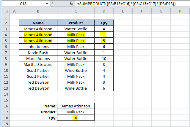
The criteria are “Name” and “Product,” and you want them to return a “Qty” value in cell C18. Because the value that you want to return is a number, you can use a simple SUMPRODUCT() formula to look for the Name “James Atkinson” and the Product “Milk Pack” to return the Qty. The SUMPRODUCT formula in cell C18 looks like this:

=SUMPRODUCT((B3:B13=C16)*(C3:C13=C17)*(D3:D13))

What it does is look in the range B3:B13 for the value in cell C16, and in the range C3:C13 for the value in cell C17. When it finds both, it returns the value in column D, from the same row where it met both criteria.  Here’s how it will look:

It returns the value 1, which corresponds to the value in cell D4 (“James Atkinson” in row 4 and also “Milk Pack” in the same row), thus returning the value in column D from that row. Let’s change the value in cell C5 from “Wine Bottle” to “Milk Pack” to see what happens with the formula in cell C18:

Because our formula found two lines where both criteria were met, it sums the values in column D in both rows, giving us a Qty of 6.

This technique cannot be used if you want to look for two criteria and return a text result. For instance, this, would not work:

You would be looking for the Name “James Atkinson” where the Qty is 1, and you’d like to return the Product name that matches these two criteria. This formula would give us a #VALUE error! Instead, you could use a formula using a combination of SUMPRODUCT, INDEX, and ROW functions, such as this one:

=INDEX(C3:C13,SUMPRODUCT((B3:B13=C16)*(D3:D13=C18)*ROW(C3:C13)),0)

You use the SUMPRODUCT function to find out the row where both criteria are met, and return the corresponding row number using the ROW function. Then you use SUMPRODUCT in the INDEX function to return the value in the array C3:C13 that is in the row number provided. The result will be like this:

You could also do this using a different technique, such as this formula in cell C17:

=LOOKUP(2,1/(B3:B13=C16)/(D3:D13=C18),(C3:C13))

The result will be the same as in the previous solution. What this formula does, is divide 1 by an array of True/False values (B3:B13=C16), and then by another array of True/False values (D3:D13=C18). This will return either 1 or a #DIV/0! error. If you use 2 as the lookup value, then the formula will match it with the last numeric value in the range, that is, the last row where both conditions are True. This is the “vector form” of the LOOKUP, so you can use it to get the corresponding value returned from C3:C13. I used 2 as the LOOKUP value, but it can be any number, starting at 1. If the formulas don’t find any match, you will, of course, get a #N/A error!

You could also use an array formula, using the MATCH function, like this:

{=INDEX(C3:C13,MATCH(1,(B3:B13=C16)*(D3:D13=C18),0))}

With this technique, you can use the MATCH function to find the row where both conditions are met. This returns a value of 1, which is matched to the 1 that is used as the lookup value of the MATCH function, thus returning us to the row where the conditions are met. Using the INDEX value, you can look for the value that is in the range C3:C13, which is in the row that was returned from the MATCH function. In this case, it was row 2, which corresponds to the second row in the range C3:C13.

Using multiple criteria to return a value from a table

All of these examples show you how to use two criteria for lookups. It’s also easy to use these formulas if you have more than two criteria-you just add them to the formulas. Here is how the formulas would look if you add one more criterion:

=SUMPRODUCT((B3:B13=C16)*(C3:C13=C17)*(E3:E13=C18)*(D3:D13))

=INDEX(C3:C13,SUMPRODUCT((B3:B13=C16)*(D3:D13=C18)*(E3:E13=C18)*ROW(C3:C13)),0)

=LOOKUP(2,1/(B3:B13=C16)/(D3:D13=C18)/(E3:E13=C18),(C3:C13))

{=INDEX(C3:C13,MATCH(1,(B3:B13=C16)*(D3:D13=C18)*(E3:E13=C18),0))}

Learn more

As you can see, depending on what’s in your data tables, you can use several different techniques using different Excel functions to look up values. Enjoy applying these to your own Excel spreadsheets.